21 challenge part 2

21.1 outliers and missing values

Here you have 3 dataframes that need cleaning. Use the methods learned in class to process the data.

import pandas as pd
import numpy as np
import matplotlib.pyplot as plt
from matplotlib.dates import DateFormatter
import matplotlib.dates as mdates
import matplotlib.ticker as ticker
import warnings
# Suppress FutureWarnings
warnings.simplefilter(action='ignore', category=FutureWarning)
warnings.simplefilter(action='ignore', category=UserWarning)
import seaborn as sns
sns.set(style="ticks", font_scale=1.5)  # white graphs, with large and legible letters

# %matplotlib widget

df1 = pd.read_csv('cleaning1.csv', 
                  index_col='date',     # set the column date as index 
                  parse_dates=True)     # turn to datetime format
df1

	A	B	C	D	E
date
2023-01-01 00:00:00	0	0.000000	0.000000	0.000000	0.000000
2023-01-01 00:05:00	1	2.245251	-1.757193	1.899602	-0.999300
2023-01-01 00:10:00	2	2.909648	0.854732	2.050146	-0.559504
2023-01-01 00:15:00	3	3.483155	0.946937	1.921080	-0.402084
2023-01-01 00:20:00	2	4.909169	0.462239	1.368470	-0.698579
...	...	...	...	...	...
2023-12-31 23:35:00	-37	1040.909898	-14808.285199	1505.020266	423.595984
2023-12-31 23:40:00	-36	1040.586547	-14808.874072	1503.915566	423.117110
2023-12-31 23:45:00	-37	1042.937417	-14808.690745	1505.479671	423.862810
2023-12-31 23:50:00	-36	1042.411572	-14809.212002	1506.174334	423.862432
2023-12-31 23:55:00	-35	1043.053520	-14809.990338	1505.767197	423.647007

105120 rows × 5 columns

df2 = pd.read_csv('cleaning2_formated.csv', 
                  index_col='datetime',     # set the column date as index 
                  parse_dates=True)     # turn to datetime format
df2

	A	B
datetime
2023-01-01 00:00:00	0.000000	0.000000
2023-01-01 01:00:00	-2.027536	0.011985
2023-01-01 02:00:00	-2.690617	-0.297928
2023-01-01 03:00:00	-1.985990	-0.309409
2023-01-01 04:00:00	-2.290898	-2.866663
...	...	...
2023-12-31 19:00:00	-74.514645	293.868086
2023-12-31 20:00:00	-74.738058	294.759346
2023-12-31 21:00:00	-75.848425	294.076349
2023-12-31 22:00:00	-77.272183	293.526461
2023-12-31 23:00:00	-76.557400	293.353369

8760 rows × 2 columns

df3 = pd.read_csv('cleaning3_formated.csv', 
                  index_col='time',     # set the column date as index 
                  parse_dates=True,     # turn to datetime format
                )
df3

	A
time
2023-01-01	0.000000
2023-01-02	-0.032027
2023-01-03	-0.586351
2023-01-04	-1.575972
2023-01-05	-2.726800
...	...
2023-12-27	6.651301
2023-12-28	6.415175
2023-12-29	7.603140
2023-12-30	8.668182
2023-12-31	8.472768

365 rows × 1 columns

21.2 cleaning df1 from outliers

21.2.1 method 1: rolling standard deviation envelope

Visual inspection of all the data:

def plot_all_columns(data):
    column_list = data.columns
    
    fig, ax = plt.subplots(len(column_list),1, sharex=True, figsize=(10,len(column_list)*2))

    if len(column_list) == 1:
        ax.plot(data[column_list[0]])
        return
    for i, column in enumerate(column_list):
        ax[i].plot(data[column])
        ax[i].set(ylabel=column)
    
    locator = mdates.AutoDateLocator(minticks=3, maxticks=7)
    formatter = mdates.ConciseDateFormatter(locator)
    ax[i].xaxis.set_major_locator(locator)
    ax[i].xaxis.set_major_formatter(formatter)

    return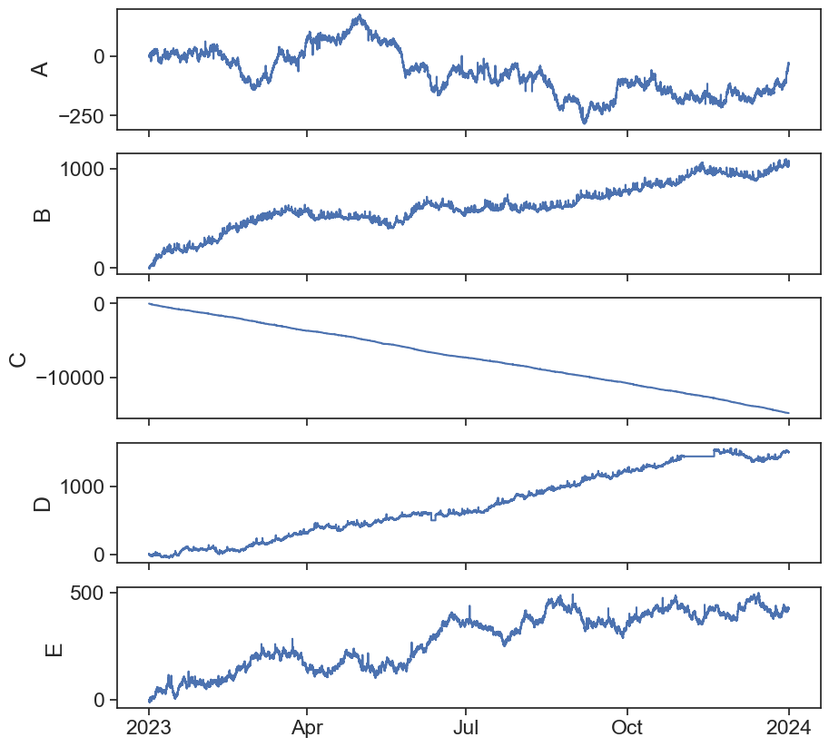

plot_all_columns(df1)

Applying the rolling std method on column A:

# find the rolling std
df1['A_std'] = df1['A'].rolling(50, center=True, min_periods=1).std()
# find the rolling mean
df1['A_mean'] = df1['A'].rolling(50, center=True, min_periods=1).mean()
# define the k parameter -> the number of standard deviations from the mean which above them we classify as outliar
k = 2
# finding the top and bottom threshold for each datapoint
df1['A_top'] = df1['A_mean'] + k*df1['A_std']
df1['A_bot'] = df1['A_mean'] - k*df1['A_std']
# creating a mask of booleans that places true if the row is an outliar and false if its not.
df1['A_out'] = ((df1['A'] > df1['A_top']) | (df1['A'] < df1['A_bot']))
# applying the mask and replacing all outliers with nans.
df1['A_filtered'] = np.where(df1['A_out'],
                                np.nan,  # use this if A_out is True
                                df1['A']) # otherwise
df1

	A	B	C	D	E	A_std	A_mean	A_top	A_bot	A_out	A_filtered
date
2023-01-01 00:00:00	0	0.000000	0.000000	0.000000	0.000000	1.262273	1.520000	4.044546	-1.004546	False	0.0
2023-01-01 00:05:00	1	2.245251	-1.757193	1.899602	-0.999300	1.331858	1.423077	4.086793	-1.240639	False	1.0
2023-01-01 00:10:00	2	2.909648	0.854732	2.050146	-0.559504	1.462738	1.296296	4.221771	-1.629179	False	2.0
2023-01-01 00:15:00	3	3.483155	0.946937	1.921080	-0.402084	1.649114	1.142857	4.441085	-2.155371	False	3.0
2023-01-01 00:20:00	2	4.909169	0.462239	1.368470	-0.698579	1.880022	0.965517	4.725561	-2.794527	False	2.0
...	...	...	...	...	...	...	...	...	...	...	...
2023-12-31 23:35:00	-37	1040.909898	-14808.285199	1505.020266	423.595984	2.988291	-32.633333	-26.656751	-38.609916	False	-37.0
2023-12-31 23:40:00	-36	1040.586547	-14808.874072	1503.915566	423.117110	3.038748	-32.655172	-26.577676	-38.732669	False	-36.0
2023-12-31 23:45:00	-37	1042.937417	-14808.690745	1505.479671	423.862810	3.077483	-32.714286	-26.559320	-38.869251	False	-37.0
2023-12-31 23:50:00	-36	1042.411572	-14809.212002	1506.174334	423.862432	3.088901	-32.814815	-26.637012	-38.992617	False	-36.0
2023-12-31 23:55:00	-35	1043.053520	-14809.990338	1505.767197	423.647007	3.128283	-32.884615	-26.628050	-39.141181	False	-35.0

105120 rows × 11 columns

21.2.2 ploting the results:

Use %matplotlib widget to visualy inspect the results.

fig, ax = plt.subplots(figsize=(10,4))

ax.plot(df1['A'], c='r', label='original')
ax.plot(df1['A_filtered'], c='b', label='filtered')
ax.plot(df1['A_bot'], c='orange',linestyle='--', label='envelope', alpha=0.5)
ax.plot(df1['A_top'], c='orange',linestyle='--', label='envelope', alpha=0.5)

ax.legend()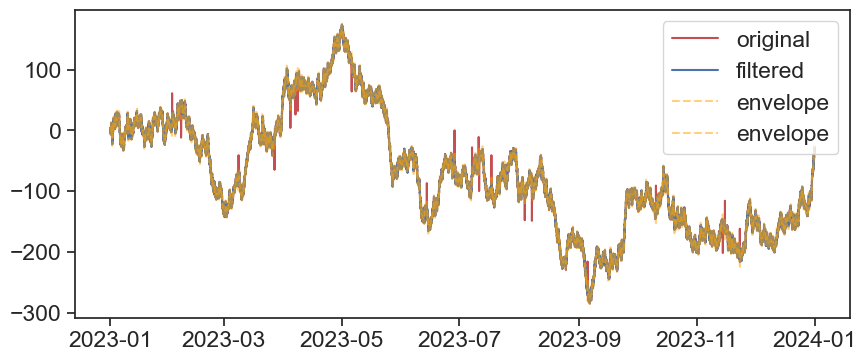

Now let’s write a function so we can easly apply it to all our data:

def rolling_std_envelop(series, window_size=50, k=2):
    series.name = 'original'
    data = series.to_frame()
    data['std'] = data['original'].rolling(window_size, center=True, min_periods=1).std()
    # find the rolling mean
    data['mean'] = data['original'].rolling(window_size, center=True, min_periods=1).mean()
    # finding the top and bottom threshold for each datapoint
    data['top'] = data['mean'] + k*data['std']
    data['bottom'] = data['mean'] - k*data['std']
    # creating a mask of booleans that places true if the row is an outliar and false if its not.
    data['outliers'] = ((data['original'] > data['top']) | (data['original'] < data['bottom']))
    # applying the mask and replacing all outliers with nans.
    data['filtered'] = np.where(data['outliers'],
                                np.nan,  # use this if outliers is True
                                data['original']) # otherwise
    return data['filtered']

Let’s test the new function:

fig, ax = plt.subplots(figsize=(10,4))

ax.plot(df1['A'], c='r', label='original')
ax.plot(rolling_std_envelop(df1['A']), c='b', label='filtered')
ax.legend()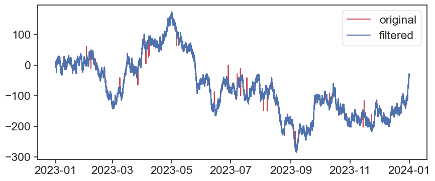

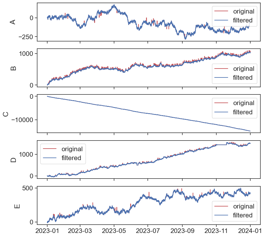
Now let’s reload df1 so it will be clean (without all the added columns from before) and apply the function on all columns:

df1 = pd.read_csv('cleaning1.csv', 
                  index_col='date',     # set the column date as index 
                  parse_dates=True)     # turn to datetime format

df1_filtered = df1.copy()
df1_filtered

	A	B	C	D	E
date
2023-01-01 00:00:00	0	0.000000	0.000000	0.000000	0.000000
2023-01-01 00:05:00	1	2.245251	-1.757193	1.899602	-0.999300
2023-01-01 00:10:00	2	2.909648	0.854732	2.050146	-0.559504
2023-01-01 00:15:00	3	3.483155	0.946937	1.921080	-0.402084
2023-01-01 00:20:00	2	4.909169	0.462239	1.368470	-0.698579
...	...	...	...	...	...
2023-12-31 23:35:00	-37	1040.909898	-14808.285199	1505.020266	423.595984
2023-12-31 23:40:00	-36	1040.586547	-14808.874072	1503.915566	423.117110
2023-12-31 23:45:00	-37	1042.937417	-14808.690745	1505.479671	423.862810
2023-12-31 23:50:00	-36	1042.411572	-14809.212002	1506.174334	423.862432
2023-12-31 23:55:00	-35	1043.053520	-14809.990338	1505.767197	423.647007

105120 rows × 5 columns

columns = df1_filtered.columns

for column in columns:
    filtered_column = rolling_std_envelop(df1_filtered[column], window_size=50, k=2)
    df1_filtered[column] = filtered_column

Now let’s plot the results:

fig, ax = plt.subplots(len(columns),1, sharex=True, figsize=(10,len(columns)*2))

for i, column in enumerate(columns):
    ax[i].plot(df1[column], c='r', label='original')
    ax[i].plot(df1_filtered[column], c='b', label='filtered')
    ax[i].legend()
    ax[i].set(ylabel=column)

21.3 plateaus

Now what about the plateaus in the series D?
That’s another form of outliers.
The following function will find rows wich have more than n equal following values and replace them with NaNs.

# function to copy paste:
def conseq_series(series, N):
    """
    part A:
    1. assume a string of 5 equal values. that's what we want to identify
    2. diff produces a string of only 4 consecutive zeros
    3. no problem, because when applying cumsum, the 4 zeros turn into a plateau of 5, that's what we want
    so far, so good
    part B:
    1. groupby value_grp splits data into groups according to cumsum.
    2. because cumsum is monotonically increasing, necessarily all groups will be composed of neighboring rows, no funny business
    3. what are those groups made of? of rows of column 'series'. this specific column is not too important, because:
    4. count 'counts' the number of elements inside each group.
    5. the real magic here is that 'transform' assigns each row of the original group with the count result.
    6. finally, we can ask the question: which rows belong to a string of identical values greater-equal than some threshold.
    zehu, you now have a mask (True-False) with the same shape as the original series.

    """
    # part A:
    sumsum_series = (
                   (series.diff() != 0)         # diff zero becomes false, otherwise true
                      .astype('int')           # true -> 1  , false -> 0
                      .cumsum()                # cumulative sum, monotonically increasing
                  )
    # part B:
    mask_outliers = (
                    series.groupby(sumsum_series)           # take original series and group it by values of cumsum
                                .transform('count')        # now count how many are in each group, assign result to each existing row. that's what transform does
                                .ge(N)                    # if row count >= than user-defined n_consecutives, assign True, otherwise False
                    )
    
    # apply mask:
    result = pd.Series(np.where(mask_outliers,
                                np.nan,  # use this if mask_outliers is True
                                series), # otherwise
                            index=series.index)
    return result

Let’s apply it to the df1_filtered df so we will end with a cleaner signal

fig, ax = plt.subplots(figsize=(10,4))
ax.plot(df1_filtered['D'], color="tab:red", label='original')
ax.plot(conseq_series(df1_filtered['D'], 10), c='tab:blue', label='filtered')
ax.set_ylabel('D')
ax.legend(frameon=False)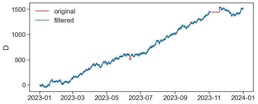

21.3.1 TO DO:

it’s not homework but you should definitely do it

Try other filtering methods
Tweak the parameters
Use other dataframes (1,2,3 and if you have your own so better)
Write custom filtering functions that you can save and use in your future work.

Yalla have fun