source: https://github.com/carloalbe/fill-large-gaps-in-timeseries-using-forecasting
import stuff
import matplotlib.pyplot as pltimport numpy as npimport pandas as pdfrom darts import TimeSeriesfrom darts.models import ExponentialSmoothing# %matplotlib widget
load data as a dataframe
= pd.read_csv('dendrometer_sample.csv' , parse_dates= ['time' ], index_col= 'time' )= df['2020-01-01' :'2020-01-31' ]= df.resample('1H' ).mean()
/var/folders/hg/vb3h0zd17wn6zfm9q5zk3pbw0000gn/T/ipykernel_22961/289532323.py:4: FutureWarning: 'H' is deprecated and will be removed in a future version, please use 'h' instead.
  df = df.resample('1H').mean()
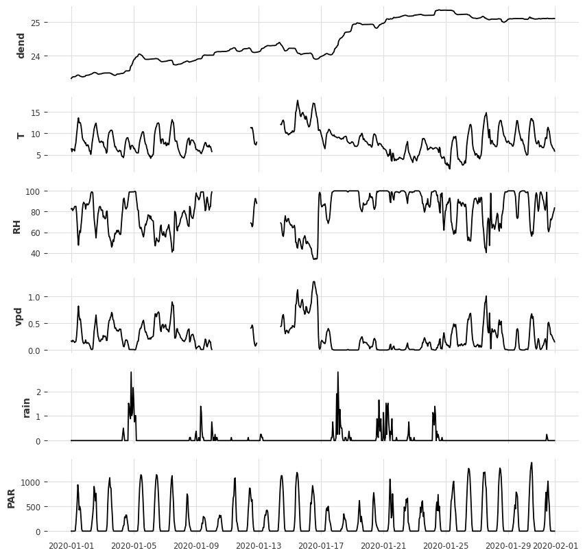
plot all columns
= df.columns= plt.subplots(len (columns), 1 , figsize= (10 , 10 ), sharex= True )for i, column in enumerate (columns):
Let’s fill the gaps in the temperature column.
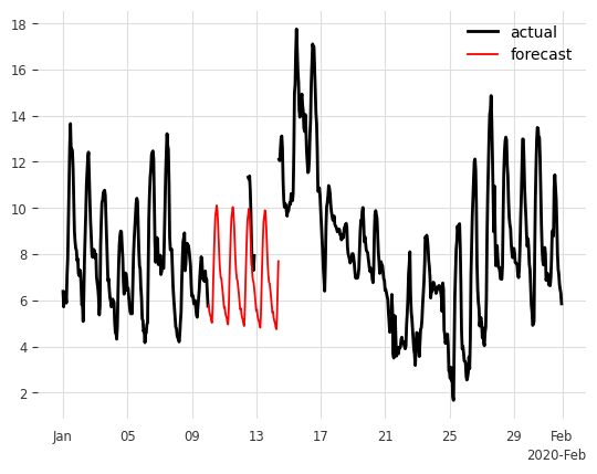
forward
Show the code
# find the time of the first nan in column 'T' = df['T' ].isnull().idxmax()# find the time of the last nan in column 'T' = df['T' ].isnull()[::- 1 ].idxmax()= pd.Timedelta('1H' )= df[first_nan:last_nan].index
/var/folders/hg/vb3h0zd17wn6zfm9q5zk3pbw0000gn/T/ipykernel_22961/4122952174.py:6: FutureWarning: 'H' is deprecated and will be removed in a future version. Please use 'h' instead of 'H'.
  one_hour = pd.Timedelta('1H')
Show the code
= TimeSeries.from_dataframe(df)= data["T" ].slice (df.index[0 ], first_nan - one_hour)
Show the code
= ExponentialSmoothing()= training_data_forward)
ExponentialSmoothing(trend=ModelMode.ADDITIVE, damped=False, seasonal=SeasonalityMode.ADDITIVE, seasonal_periods=None, random_state=0, kwargs=None)
Show the code
= int ((last_nan - first_nan) / one_hour) + 1 = model_forward.predict(n= N_to_fill); = pd.Series(data= prediction.values().flatten(), index= missing_index)
Show the code
= plt.subplots()'T' ].plot(label= 'actual' )# prediction.plot(label='forecast', lw=2) = 'red' , label= 'forecast' )set (xlabel= "" )
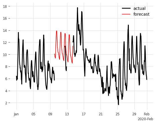
backward
Show the code
= data["T" ].slice (last_nan + one_hour, df.index[- 1 ])= training_data2.time_index= training_data2.values()= values[::- 1 ]= TimeSeries.from_times_and_values(time_index, reversed_values)
Show the code
= ExponentialSmoothing()= training_data_backward)
ExponentialSmoothing(trend=ModelMode.ADDITIVE, damped=False, seasonal=SeasonalityMode.ADDITIVE, seasonal_periods=None, random_state=0, kwargs=None)
Show the code
= model_backward.predict(n= N_to_fill)= pd.Series(data= prediction2.values().flatten()[::- 1 ], index= missing_index)
Show the code
= plt.subplots()'T' ].plot(label= 'actual' )= 'red' , label= 'forecast' )set (xlabel= "" )
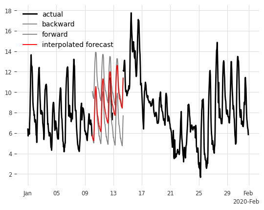
interpolate
Show the code
= np.linspace(1 , 0 , N_to_fill)= df_pred_forward * ramp + df_pred_backward * (1 - ramp)
Show the code
= plt.subplots()'T' ].plot(label= 'actual' )# prediction.plot(label='forecast', lw=2) = 'red' , label= 'interpolated forecast' )set (xlabel= "" )
Show the code
= plt.subplots()'T' ].plot(label= 'actual' )= 'gray' , label= 'backward' )= 'gray' , label= 'forward' )= 'red' , label= 'interpolated forecast' )set (xlabel= "" )