65 assignment 3
In this assignment, you will incorporate all that you have learned until now on real data! Often in homework, teachers (including us) tailor-make a dataset to practice the subjects studied in class. This example is not tailored-made; it’s from real life, yet it showcases the importance and relevance of all the subjects studied till now.
65.1 background
A tree in Boston is being continuously measured, using an IoT box created by me (Erez).
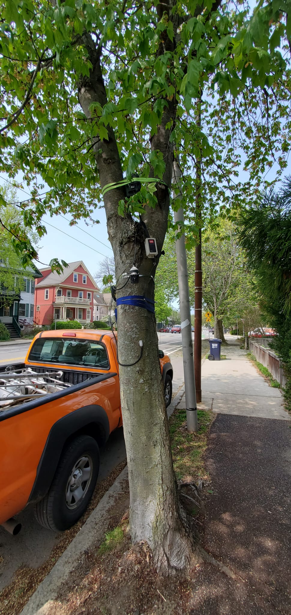
Sensors connected to this box measure the following
- Air temperature (C)
- Air relative humidity (%)
- Change of tree circumference (\mum) measured by a dendrometer
- Battery voltage (V)
- Internal temperature (°C) (inside the box)
The box collects data from sensors every 30 minutes and uploads them to the cloud once a day. The cloud server puts a time stamp on every datapoint, but to make sure things are right: the timestamp at the time of data collection is uploaded as a variable (in units of UNIX at GMT).
You can see the box’s dashboard here.
Download the file boston_raw.csv here.
Here is a break down of the columns:
created_at- Time stamp added by the cloudentry_id- Index added by the cloudfield1- Change of tree circumference (\mum)field2- Air temperature (°C)field3- Air relative humidity (%)field4- Battery voltage (V)field5- Internal temperature (c) (inside the box)field6- True timestamp (in units of UNIX at GMT)latitude- Emptylongitude- Emptyelevation- Emptystatus- Empty
65.2 analysis
Follow the instructions below to process the data.
Make sure your text answers are in markdown cells and are numbered. Text answers in Python cells might be ignored.
Upload to Moodle the completed operational (no errors) Jupyter Notebook file (.ipynb), along with the boston_raw.csv file.
Load
csvto a dataframe.Rename the columns to short and convenient names that make sense for you.
Convert the UNIX time stamp to a human-readable time stamp. Don’t forget to convert the time zone from GMT to Boston.
Set the new converted timestamp as the index.
Sort the entire dataframe based on the chronological order of the index. Here is an example code:
df.sort_index(inplace=True)Plot all columns and explore the data. Zoom in. Do you see gaps? Outliers? Jumps? Don’t process them yet. Make a list of 3 things you see.
Bonus: Identify any patterns related to outliers/gaps and explain their occurrence.Count how many
nanvalues are in each column.Now take a look at the datetime index. As noted earlier, the readings on the device are every 30 minutes, but is that what we see in the data? Do we have a continuous datetime index where every index is 30 min apart? Are there gaps? Are the timestamps consistent? Is there a drift (e.g. sometimes the data comes in at 00:30 and sometimes 00:27 or 00:20, etc..). Explain.
Think about a quick and dirty fix to this problem. Then read below:
- An easy fix will be to resample the data at
30Tand take the mean. That will ensure consistent timestamps and no gaps (in the index). - Why quick and “dirty”? What is dirty about it? is there a problem? Explain.
- Anyway, we will continue with this. There are other ways but they are a bit more complex.
- An easy fix will be to resample the data at
Re-count the number of
nanvalues in each column. Explain any changes observed.Now that the index is consistent and without gaps, we want to all data (fix jumps, remove outliers and fill gaps).
- I’ll start with a hint regarding the dendrometer that requires some background knowledge you may not know. The dendrometer has a metal band wrapping the trunk of the tree and it needs to be reset when the sensor readings are approaching the limit of 60,000 \mum. So you can see it in the data that someone reset the band some day in September. What needs to be done is to shift up all the data after the jump to be a continuation of the data before the jump. Plot the dendrometer data after the shift.
Outliers: show results of at least 2 methods of outlier identification applied to the data. Compare them and choose the one that did the best work and explain. Outliers should be replaced with
nanvalues.Filling gaps (missing values): show results of at least 2 methods of gap filling. Compare them and choose the one that did the best work and explain. Differently from what we learned during class, this time we don’t have the real data to compare to. Bonus: you might find a way to download data from Boston from a meteorological station, and compare to our data.
At this point the data should be clean (no outliers or gaps) in all columns and ready for exploration.
Add a column of vapor pressure deficit (VPD) based on the air temperature and relative humidity. The formula can be found here.
Using the toolkit learned in the course (for example: smoothing, seasonal decompose, detrending, etc..) show the following:
- How temperature affects dendrometer readings (hint, this happens in a large time scale of months). Showing it graphically is enough! No need to prove it statistically (for example don’t apply correlation).
- How VPD affects tree dendrometer readings (hint, this happens in a small time scale of days, during the hotter months). Showing it graphically is enough! No need to prove it statistically (for example don’t apply correlation).