22 challenge

22.1 Importing Bad .csv Files

Here we will get a taste of what it feels like to work with bad .csv files and how to fix them.

TO DO:

Create a folder for this challenge, name it whatever you want.
Download this Jupyter notebook and move it to that folder.
Download these 3 .csv files and part 2 notebook:
1. cleaning1
2. cleaning2-
3. cleaning3
4. Go to challenge part 2 and download it from there.
Move these files into your folder.

22.1.1 Import

import pandas as pd
import numpy as np
import matplotlib.pyplot as plt
from matplotlib.dates import DateFormatter
import matplotlib.dates as mdates
import matplotlib.ticker as ticker
import warnings
# Suppress FutureWarnings
warnings.simplefilter(action='ignore', category=FutureWarning)
warnings.simplefilter(action='ignore', category=UserWarning)
import seaborn as sns
sns.set(style="ticks", font_scale=1.5)  # white graphs, with large and legible letters

# %matplotlib widget

22.2 dataset 1

df1 = pd.read_csv('cleaning1.csv')
df1

	date	A	B	C	D	E
0	2023-01-01 00:00:00	0	0.000000	0.000000	0.000000	0.000000
1	2023-01-01 00:05:00	1	2.245251	-1.757193	1.899602	-0.999300
2	2023-01-01 00:10:00	2	2.909648	0.854732	2.050146	-0.559504
3	2023-01-01 00:15:00	3	3.483155	0.946937	1.921080	-0.402084
4	2023-01-01 00:20:00	2	4.909169	0.462239	1.368470	-0.698579
...	...	...	...	...	...	...
105115	2023-12-31 23:35:00	-37	1040.909898	-14808.285199	1505.020266	423.595984
105116	2023-12-31 23:40:00	-36	1040.586547	-14808.874072	1503.915566	423.117110
105117	2023-12-31 23:45:00	-37	1042.937417	-14808.690745	1505.479671	423.862810
105118	2023-12-31 23:50:00	-36	1042.411572	-14809.212002	1506.174334	423.862432
105119	2023-12-31 23:55:00	-35	1043.053520	-14809.990338	1505.767197	423.647007

105120 rows × 6 columns

Now let’s put the column ‘date’ in the index with datetime format

# we can change the format of the column to datetime and then set it as the index.
df1['date'] = pd.to_datetime(df1['date'])
df1.set_index('date', inplace=True)
df1

	A	B	C	D	E
date
2023-01-01 00:00:00	0	0.000000	0.000000	0.000000	0.000000
2023-01-01 00:05:00	1	2.245251	-1.757193	1.899602	-0.999300
2023-01-01 00:10:00	2	2.909648	0.854732	2.050146	-0.559504
2023-01-01 00:15:00	3	3.483155	0.946937	1.921080	-0.402084
2023-01-01 00:20:00	2	4.909169	0.462239	1.368470	-0.698579
...	...	...	...	...	...
2023-12-31 23:35:00	-37	1040.909898	-14808.285199	1505.020266	423.595984
2023-12-31 23:40:00	-36	1040.586547	-14808.874072	1503.915566	423.117110
2023-12-31 23:45:00	-37	1042.937417	-14808.690745	1505.479671	423.862810
2023-12-31 23:50:00	-36	1042.411572	-14809.212002	1506.174334	423.862432
2023-12-31 23:55:00	-35	1043.053520	-14809.990338	1505.767197	423.647007

105120 rows × 5 columns

If we know that in advance, we can write everything in one command when we import the csv.

df1 = pd.read_csv('cleaning1.csv', 
                  index_col='date',     # set the column date as index 
                  parse_dates=True)     # turn to datetime format
df1

	A	B	C	D	E
date
2023-01-01 00:00:00	0	0.000000	0.000000	0.000000	0.000000
2023-01-01 00:05:00	1	2.245251	-1.757193	1.899602	-0.999300
2023-01-01 00:10:00	2	2.909648	0.854732	2.050146	-0.559504
2023-01-01 00:15:00	3	3.483155	0.946937	1.921080	-0.402084
2023-01-01 00:20:00	2	4.909169	0.462239	1.368470	-0.698579
...	...	...	...	...	...
2023-12-31 23:35:00	-37	1040.909898	-14808.285199	1505.020266	423.595984
2023-12-31 23:40:00	-36	1040.586547	-14808.874072	1503.915566	423.117110
2023-12-31 23:45:00	-37	1042.937417	-14808.690745	1505.479671	423.862810
2023-12-31 23:50:00	-36	1042.411572	-14809.212002	1506.174334	423.862432
2023-12-31 23:55:00	-35	1043.053520	-14809.990338	1505.767197	423.647007

105120 rows × 5 columns

Now let’s plot all the columns and see what we have.

def plot_all_columns(data):
    column_list = data.columns
    
    fig, ax = plt.subplots(len(column_list),1, sharex=True, figsize=(10,len(column_list)*2))

    if len(column_list) == 1:
        ax.plot(data[column_list[0]])
        return
    for i, column in enumerate(column_list):
        ax[i].plot(data[column])
        ax[i].set(ylabel=column)
    
    locator = mdates.AutoDateLocator(minticks=3, maxticks=7)
    formatter = mdates.ConciseDateFormatter(locator)
    ax[i].xaxis.set_major_locator(locator)
    ax[i].xaxis.set_major_formatter(formatter)

    return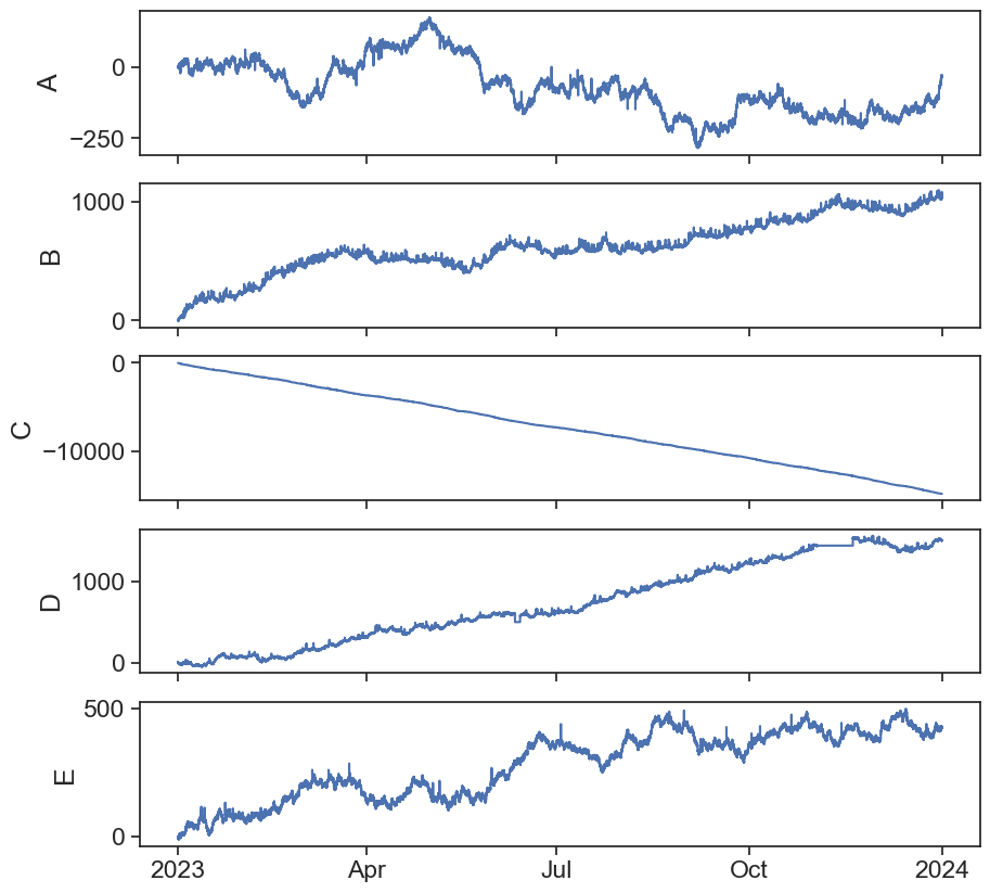

plot_all_columns(df1)

Looks like some of this data needs cleaning…

22.3 dataset 2

df2 = pd.read_csv('cleaning2-.csv')
df2

	A B date time
0	0.0 0.0 01012023 00:00:00
1	-2.0275363548598184 0.011984922825112581 01012...
2	-2.690616715983192 -0.29792822981957684 010120...
3	-1.9859899758267612 -0.30940867922490206 01012...
4	-2.290897621584889 -2.8666633353521624 0101202...
...	...
8755	-74.51464473079395 293.8680858227996 31122023 ...
8756	-74.73805809332175 294.7593463919649 31122023 ...
8757	-75.84842465358788 294.07634907736116 31122023...
8758	-77.27218272637339 293.526461290973 31122023 2...
8759	-76.55739976945038 293.35336890454107 31122023...

8760 rows × 1 columns

Something is wrong…
Let’s open the actual .csv file and take a quick look.
It seems that the values are separated by spaces and not by commas ,.

df2 = pd.read_csv('cleaning2-.csv', delimiter=' ')
df2

	A	B	date	time
0	0.000000	0.0	1012023	00:00:00
1	-2.027536	0.011984922825112581	1012023	01:00:00
2	-2.690617	-0.29792822981957684	1012023	02:00:00
3	-1.985990	-0.30940867922490206	1012023	03:00:00
4	-2.290898	-2.8666633353521624	1012023	04:00:00
...	...	...	...	...
8755	-74.514645	293.8680858227996	31122023	19:00:00
8756	-74.738058	294.7593463919649	31122023	20:00:00
8757	-75.848425	294.07634907736116	31122023	21:00:00
8758	-77.272183	293.526461290973	31122023	22:00:00
8759	-76.557400	293.35336890454107	31122023	23:00:00

8760 rows × 4 columns

# convert the date column to datetime
df2['date_corrected'] = pd.to_datetime(df2['date'])
# df2['date_corrected'] = pd.to_datetime(df2['date'], format='%d%m%Y')

df2

	A	B	date	time	date_corrected
0	0.000000	0.0	1012023	00:00:00	1970-01-01 00:00:00.001012023
1	-2.027536	0.011984922825112581	1012023	01:00:00	1970-01-01 00:00:00.001012023
2	-2.690617	-0.29792822981957684	1012023	02:00:00	1970-01-01 00:00:00.001012023
3	-1.985990	-0.30940867922490206	1012023	03:00:00	1970-01-01 00:00:00.001012023
4	-2.290898	-2.8666633353521624	1012023	04:00:00	1970-01-01 00:00:00.001012023
...	...	...	...	...	...
8755	-74.514645	293.8680858227996	31122023	19:00:00	1970-01-01 00:00:00.031122023
8756	-74.738058	294.7593463919649	31122023	20:00:00	1970-01-01 00:00:00.031122023
8757	-75.848425	294.07634907736116	31122023	21:00:00	1970-01-01 00:00:00.031122023
8758	-77.272183	293.526461290973	31122023	22:00:00	1970-01-01 00:00:00.031122023
8759	-76.557400	293.35336890454107	31122023	23:00:00	1970-01-01 00:00:00.031122023

8760 rows × 5 columns

# df2['date_corrected'] = pd.to_datetime(df2['date'][:780], format='%d%m%Y')
# df2['date_corrected'] = pd.to_datetime(df2['date'][780:800], format='%d%m%Y')
# df2['date'][780:800]

data_types = {'date': str , 'time':str}

# Read the CSV file with specified data types
df2 = pd.read_csv('cleaning2-.csv', delimiter=' ', dtype=data_types)
df2

	A	B	date	time
0	0.000000	0.0	01012023	00:00:00
1	-2.027536	0.011984922825112581	01012023	01:00:00
2	-2.690617	-0.29792822981957684	01012023	02:00:00
3	-1.985990	-0.30940867922490206	01012023	03:00:00
4	-2.290898	-2.8666633353521624	01012023	04:00:00
...	...	...	...	...
8755	-74.514645	293.8680858227996	31122023	19:00:00
8756	-74.738058	294.7593463919649	31122023	20:00:00
8757	-75.848425	294.07634907736116	31122023	21:00:00
8758	-77.272183	293.526461290973	31122023	22:00:00
8759	-76.557400	293.35336890454107	31122023	23:00:00

8760 rows × 4 columns

df2['date_corrected'] = pd.to_datetime(df2['date'], format='%d%m%Y')
df2

	A	B	date	time	date_corrected
0	0.000000	0.0	01012023	00:00:00	2023-01-01
1	-2.027536	0.011984922825112581	01012023	01:00:00	2023-01-01
2	-2.690617	-0.29792822981957684	01012023	02:00:00	2023-01-01
3	-1.985990	-0.30940867922490206	01012023	03:00:00	2023-01-01
4	-2.290898	-2.8666633353521624	01012023	04:00:00	2023-01-01
...	...	...	...	...	...
8755	-74.514645	293.8680858227996	31122023	19:00:00	2023-12-31
8756	-74.738058	294.7593463919649	31122023	20:00:00	2023-12-31
8757	-75.848425	294.07634907736116	31122023	21:00:00	2023-12-31
8758	-77.272183	293.526461290973	31122023	22:00:00	2023-12-31
8759	-76.557400	293.35336890454107	31122023	23:00:00	2023-12-31

8760 rows × 5 columns

df2['datetime'] = pd.to_datetime(df2['date'] + ' ' + df2['time'], format='%d%m%Y %H:%M:%S')
df2

	A	B	date	time	date_corrected	datetime
0	0.000000	0.0	01012023	00:00:00	2023-01-01	2023-01-01 00:00:00
1	-2.027536	0.011984922825112581	01012023	01:00:00	2023-01-01	2023-01-01 01:00:00
2	-2.690617	-0.29792822981957684	01012023	02:00:00	2023-01-01	2023-01-01 02:00:00
3	-1.985990	-0.30940867922490206	01012023	03:00:00	2023-01-01	2023-01-01 03:00:00
4	-2.290898	-2.8666633353521624	01012023	04:00:00	2023-01-01	2023-01-01 04:00:00
...	...	...	...	...	...	...
8755	-74.514645	293.8680858227996	31122023	19:00:00	2023-12-31	2023-12-31 19:00:00
8756	-74.738058	294.7593463919649	31122023	20:00:00	2023-12-31	2023-12-31 20:00:00
8757	-75.848425	294.07634907736116	31122023	21:00:00	2023-12-31	2023-12-31 21:00:00
8758	-77.272183	293.526461290973	31122023	22:00:00	2023-12-31	2023-12-31 22:00:00
8759	-76.557400	293.35336890454107	31122023	23:00:00	2023-12-31	2023-12-31 23:00:00

8760 rows × 6 columns

df2.drop(columns=['date', 'time', 'date_corrected'], inplace=True)
df2.set_index('datetime', inplace=True)
df2

	A	B
datetime
2023-01-01 00:00:00	0.000000	0.0
2023-01-01 01:00:00	-2.027536	0.011984922825112581
2023-01-01 02:00:00	-2.690617	-0.29792822981957684
2023-01-01 03:00:00	-1.985990	-0.30940867922490206
2023-01-01 04:00:00	-2.290898	-2.8666633353521624
...	...	...
2023-12-31 19:00:00	-74.514645	293.8680858227996
2023-12-31 20:00:00	-74.738058	294.7593463919649
2023-12-31 21:00:00	-75.848425	294.07634907736116
2023-12-31 22:00:00	-77.272183	293.526461290973
2023-12-31 23:00:00	-76.557400	293.35336890454107

8760 rows × 2 columns

plot_all_columns(df2)

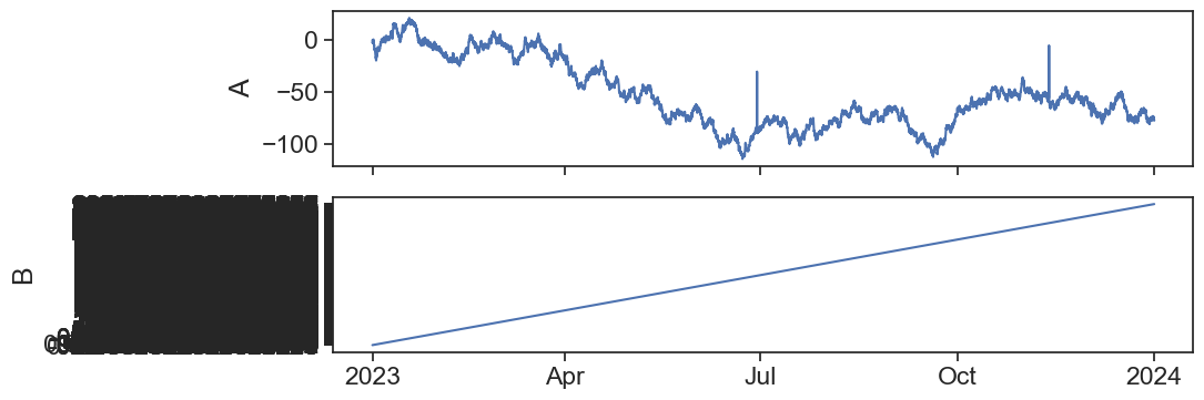
What happened in the second ax?

df2.dtypes

A    float64
B     object
dtype: object

# use pd.to_numeric to convert column 'B' to float
df2['B'] = pd.to_numeric(df2['B'],
                          errors='coerce'  # 'coerce' will convert non-numeric values to NaN if they can't be converted
                          )
df2.dtypes

A    float64
B    float64
dtype: object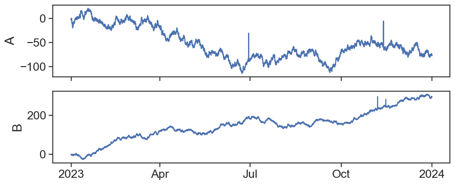

plot_all_columns(df2)

data_types = {'date': str , 'time':str}

# Read the CSV file with specified data types
df2 = pd.read_csv('cleaning2-.csv', delimiter=' ', dtype=data_types, na_values='-')
df2['datetime'] = pd.to_datetime(df2['date'] + ' ' + df2['time'], format='%d%m%Y %H:%M:%S')
df2.drop(columns=['date', 'time'], inplace=True)
df2.set_index('datetime', inplace=True)
df2

	A	B
datetime
2023-01-01 00:00:00	0.000000	0.000000
2023-01-01 01:00:00	-2.027536	0.011985
2023-01-01 02:00:00	-2.690617	-0.297928
2023-01-01 03:00:00	-1.985990	-0.309409
2023-01-01 04:00:00	-2.290898	-2.866663
...	...	...
2023-12-31 19:00:00	-74.514645	293.868086
2023-12-31 20:00:00	-74.738058	294.759346
2023-12-31 21:00:00	-75.848425	294.076349
2023-12-31 22:00:00	-77.272183	293.526461
2023-12-31 23:00:00	-76.557400	293.353369

8760 rows × 2 columns

df2.to_csv('cleaning2_formated.csv')

22.4 dataset 3

df3 = pd.read_csv('cleaning3.csv')
df3

	#
0	# data created by
1	# Yair Mau
2	# for time series data analysis
3	#
4	# time format: unix (s)
...	...
370	6.651300774019661 1703635200.0
371	6.4151748349408715 1703721600.0
372	7.603140054178304 1703808000.0
373	8.668182044560869 1703894400.0
374	8.472767724946076 1703980800.0

375 rows × 1 columns

Again, let’s look at the actual .csv file.

df3 = pd.read_csv('cleaning3.csv', comment='#')
df3

	A time
0	0.0 1672531200.0
1	-0.03202661701444382 1672617600.0
2	-0.5863508675173621 1672704000.0
3	-1.5759721567247762 1672790400.0
4	-2.7267995149281266 1672876800.0
...	...
360	6.651300774019661 1703635200.0
361	6.4151748349408715 1703721600.0
362	7.603140054178304 1703808000.0
363	8.668182044560869 1703894400.0
364	8.472767724946076 1703980800.0

365 rows × 1 columns

df3 = pd.read_csv('cleaning3.csv', comment='#', delimiter=' ')
df3

	A	time
0	0.000000	1.672531e+09
1	-0.032027	1.672618e+09
2	-0.586351	1.672704e+09
3	-1.575972	1.672790e+09
4	-2.726800	1.672877e+09
...	...	...
360	6.651301	1.703635e+09
361	6.415175	1.703722e+09
362	7.603140	1.703808e+09
363	8.668182	1.703894e+09
364	8.472768	1.703981e+09

365 rows × 2 columns

df3.dtypes

A       float64
time    float64
dtype: object

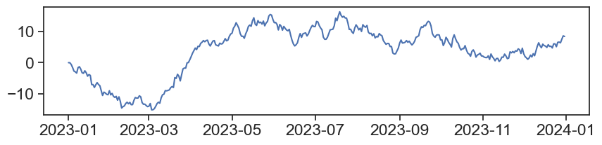
Time is in unix.
unix converter

print(df3['time'][0])

1672531200.0

df3['time'] = pd.to_datetime(df3['time'], unit='s')
df3.set_index('time', inplace=True)
df3

	A
time
2023-01-01	0.000000
2023-01-02	-0.032027
2023-01-03	-0.586351
2023-01-04	-1.575972
2023-01-05	-2.726800
...	...
2023-12-27	6.651301
2023-12-28	6.415175
2023-12-29	7.603140
2023-12-30	8.668182
2023-12-31	8.472768

365 rows × 1 columns

df3 = pd.read_csv('cleaning3.csv', 
                  index_col='time',     # set the column date as index 
                  parse_dates=True,     # turn to datetime format
                  comment='#', 
                  delimiter=' ')
df3.index = pd.to_datetime(df3.index, unit='s')
df3

	A
time
2023-01-01	0.000000
2023-01-02	-0.032027
2023-01-03	-0.586351
2023-01-04	-1.575972
2023-01-05	-2.726800
...	...
2023-12-27	6.651301
2023-12-28	6.415175
2023-12-29	7.603140
2023-12-30	8.668182
2023-12-31	8.472768

365 rows × 1 columns

plot_all_columns(df3)

df3.to_csv('cleaning3_formated.csv')