40  Fourier transform

40.1 basic wave concepts

The function

f(t) = B\sin(2\pi f t) \tag{40.1}

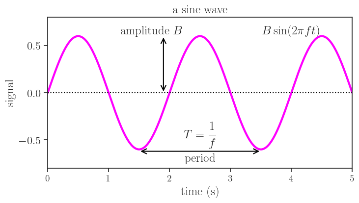
has two basic characteristics, its amplitude B and frequency f.

import stuff
import numpy as np
import matplotlib.pyplot as plt
import seaborn as sns
import matplotlib as mpl
sns.set(style="ticks", font_scale=1.5)

# %matplotlib widget

# Configure Matplotlib to use LaTeX font
plt.rcParams.update({
    "xtick.labelsize": 14,
    "text.usetex": True,
    "font.family": "serif",
    "font.serif": ["Computer Modern Roman"]
})
data to plot
T = 2.0  # s
f = 1.0 / T
n_periods = 2.5
dt = 0.01
B = 0.6
t = np.arange(0, T*n_periods + dt, dt)
s = B * np.sin(2.0 * np.pi * f * t)
c = B * np.cos(2.0 * np.pi * f * t)
plot
fig, ax = plt.subplots(figsize=(8,4))
ax.plot(t, s, color="magenta", lw=3)
ax.plot(t, 0*t, color="black", ls=":")
ax.annotate("",
            xy=(1.9, 0.0), xycoords='data',
            xytext=(1.9, 0.6), textcoords='data',
            color="black",
            arrowprops=dict(arrowstyle="<->",
                            connectionstyle="arc3",
                            color="black",
                            lw=1.5),
            )
ax.annotate("",
            xy=(1.5, -0.62), xycoords='data',
            xytext=(3.5, -0.62), textcoords='data',
            color="black",
            arrowprops=dict(arrowstyle="<->",
                            connectionstyle="arc3",
                            color="black",
                            lw=1.5),
            )
ax.text(1.7, 0.62, r"amplitude $B$", ha="center")
ax.text(2.5, -0.73, r"period", ha="center")
ax.text(2.5, -0.48, r"$T=\displaystyle\frac{1}{f}$", ha="center")
ax.text(4.0, 0.62, r"$B\sin(2\pi ft)$", ha="center")
ax.set(xlim=[t[0], t[-1]],
       ylim=[-0.8, 0.8],
       title="a sine wave",
       xlabel="time (s)",
       ylabel="signal");
# fig.savefig("sine1.png", dpi=300, bbox_inches="tight")

In the figure above, the amplitude B=0.6 and we see that the distance between two peaks is called period, T=2 s. The frequency is defined as the inverse of the period:

f = \frac{1}{T}. \tag{40.2}

When time is in seconds, then the frequency is measured in Hertz (Hz). For the graph above, therefore, we see a wave whose frequency is f = 1/(2 \text{ s}) = 0.5 Hz.

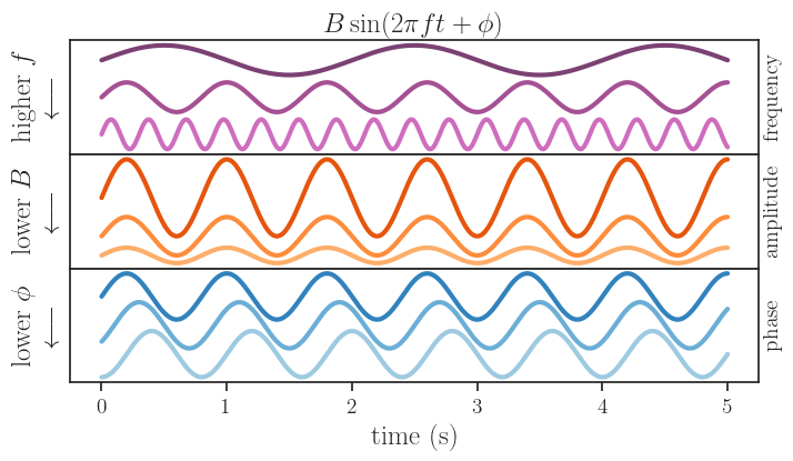
In the figure below, we see what happens when we vary the values of the frequency and amplitude.

Show the code
t20b = mpl.colormaps['tab20b']
t20c = mpl.colormaps['tab20c']

fig, ax = plt.subplots(3, 1, figsize=(8,4), sharex=True)
fig.subplots_adjust(
                    hspace=0.0, wspace=0.02)
A = 0.4

s = A * np.sin(2.0 * np.pi * (1/2.0) * t)
ax[0].plot(t, s, color=t20b.colors[16], lw=3)
s = A * np.sin(2.0 * np.pi * (1/0.8) * t) - 1
ax[0].plot(t, s, color=t20b.colors[17], lw=3)
s = A * np.sin(2.0 * np.pi * (1/0.3) * t) - 2
ax[0].plot(t, s, color=t20b.colors[18], lw=3)

s = 1 * np.sin(2.0 * np.pi * (1/0.8) * t)
ax[1].plot(t, s, color=t20c.colors[4], lw=3)
s = 0.5 * np.sin(2.0 * np.pi * (1/0.8) * t) - 1
ax[1].plot(t, s, color=t20c.colors[5], lw=3)
s = 0.2 * np.sin(2.0 * np.pi * (1/0.8) * t) - 1.5
ax[1].plot(t, s, color=t20c.colors[6], lw=3)

s = A * np.sin(2.0 * np.pi * (1/0.8) * t)
ax[2].plot(t, s, color=t20c.colors[0], lw=3)
s = A * np.sin(2.0 * np.pi * (1/0.8) * t - np.pi/4) - 0.5
ax[2].plot(t, s, color=t20c.colors[1], lw=3)
s = A * np.sin(2.0 * np.pi * (1/0.8) * t - 2*np.pi/4) - 1
ax[2].plot(t, s, color=t20c.colors[2], lw=3)

ax[0].text(1.02, 0.5, "frequency", transform=ax[0].transAxes,
         horizontalalignment='center', verticalalignment='center',
         fontweight="bold", fontsize=14,
         rotation=90)
ax[1].text(1.02, 0.5, "amplitude", transform=ax[1].transAxes,
         horizontalalignment='center', verticalalignment='center',
         fontweight="bold", fontsize=14,
         rotation=90)
ax[2].text(1.02, 0.5, "phase", transform=ax[2].transAxes,
         horizontalalignment='center', verticalalignment='center',
         fontweight="bold", fontsize=14,
         rotation=90)


ax[0].set(title=r"$B\sin(2\pi ft+\phi)$",
          yticks=[],
          ylabel=r"higher $f$"+"\n"+r"$\longleftarrow$")
ax[1].set(yticks=[],
          ylabel=r"lower $B$"+"\n"+r"$\longleftarrow$")
ax[2].set(xlabel="time (s)",
          yticks=[],
          ylabel=r"lower $\phi$"+"\n"+r"$\longleftarrow$");
# fig.savefig("sine2.png", dpi=300, bbox_inches="tight")

The graph above introduces two new characteristics of a wave, its phase \phi, and its offset B. A more general description of a sine wave is

f(t) = B\sin(2\pi f t + \phi) + B_0. \tag{40.3}

The offset B_0 moves the wave up and down, while changing the value of \phi makes the sine wave move left and right. When the phase \phi=2\pi, the sine wave will have shifted a full period, and the resulting wave is identical to the original:

B\sin(2\pi f t) = B\sin(2\pi f t + 2\pi). \tag{40.4}

All the above can also be said about a cosine, whose general form can be given as

A\cos(2\pi f t + \phi) + A_0 \tag{40.5}

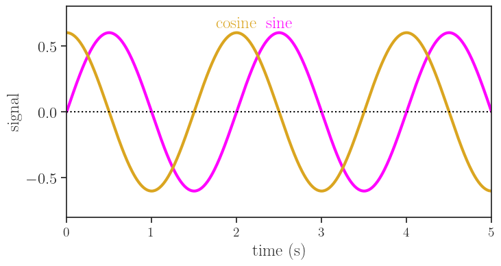
One final point before we jump into the deep waters is that the sine and cosine functions are related through a simple phase shift:

\cos\left(2\pi f t + \frac{\pi}{2}\right) = \sin\left(2\pi f t\right)

plot sine and cosine
fig, ax = plt.subplots(figsize=(8,4))
ax.plot(t, s, color="magenta", lw=3)
ax.plot(t, c, color="goldenrod", lw=3)
ax.plot(t, 0*t, color="black", ls=":")
ax.text(2.5, 0.64, "sine", ha="center", color="magenta")
ax.text(2.0, 0.64, "cosine", ha="center", color="goldenrod")
ax.set(xlim=[t[0], t[-1]],
       ylim=[-0.8, 0.8],
       xlabel="time (s)",
       ylabel="signal");

40.2 Fourier’s theorem

Fourier’s theorem states that

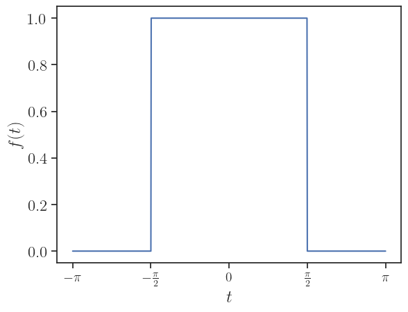
Any periodic signal is composed of a superposition of pure sine waves, with suitably chosen amplitudes and phases, whose frequencies are harmonics of the fundamental frequency of the signal.

40.3 Fourier series

a periodic function can be described as a sum of sines and cosines.

The most common way of representing the Fourier series is f(t) = \frac{1}{2}a_0 + \sum_{n=1}^{\infty}a_n\cos(nt) + \sum_{n=1}^{\infty}b_n\sin(nt) \tag{40.6}

for a periodic function f(t) in the interval -\pi<t<\pi, where

\begin{split} a_0 &= \frac{1}{\pi}\int_{-\pi}^{\pi}f(t)dt\\ a_n &= \frac{1}{\pi}\int_{-\pi}^{\pi}f(t)\cos(nt)dt\\ b_n &= \frac{1}{\pi}\int_{-\pi}^{\pi}f(t)\sin(nt)dt\\ \end{split} \tag{40.7}

Let’s see some excellent visual demonstrations. The classic examples are usually the square function and the sawtooth function:

Source: https://www.geogebra.org/m/tkajbzmg

Source: https://www.geogebra.org/m/k4eq4fkr

We can take advantage of complex numbers to rewrite the Fourier series in a more compact and elegant way:

f(t) = \sum_{n=-\infty}^{\infty} c_n e^{2\pi i \frac{n}{P} t}

for a periodic function between -\frac{P}{2}\le t \le\frac{P}{2}, and the coefficients are given by

c_n = \frac{1}{P}\int_{-\frac{P}{2}}^{\frac{P}{2}}f(t) e^{- 2\pi i \frac{n}{P} t}dt.

If you are not familiar with complex numbers, or you need a refresher, visit Dennis Sun’s excellent “Introduction to Probability” webpage.

The series expressed as a sum of sines and cosines could be translated into an expression of a complex exponential by taking advantage of Euler’s formula:

e^{ix} = \cos(x) + i\sin(x)

40.4 Fourier transform

This is a generalization of a Fourier series, but for non-periodic signals. If we take the limit P\rightarrow\infty in the equations above, we have that

f(t) = \int_{-\infty}^{\infty} F(k) e^{2\pi i k t}dk,

where F(k) now takes the role of the coefficients from before, and it is given by

F(k) = \int_{-\infty}^{\infty} f(t) e^{-2\pi i k t}dk.

If t is in seconds, the frequency k is given in Hertz (Hz).

See the following animations to visualize the theorem in action.

Fourier series and transform.gif
Source: https://en.wikipedia.org/wiki/File:Fourier_series_and_transform.gif

Fourier synthesis square wave animated
Source: https://commons.wikimedia.org/wiki/File:Fourier_synthesis_square_wave_animated.gif

Sawtooth Fourier Animation
Source: https://commons.wikimedia.org/wiki/File:Sawtooth_Fourier_Animation.gif

Continuous Fourier transform of rect and sinc functions
Source: Wikimedia

40.5 fun calculation of a Fourier series

Let’s calculate the Fourier series of the periodic function f(t) over the domain -\pi<t<\pi:

f(t)= \begin{cases} 1, & \text{if } -\frac{\pi}{2}<t<\frac{\pi}{2}\\ 0, & \text{otherwise} \end{cases}

Show the code
pi = np.pi
t = np.linspace(-pi,pi,1001)
f = np.zeros(len(t))
mask = np.where(np.abs(t)<pi/2)
f[mask] = 1.0

fig, ax = plt.subplots()
ax.plot(t, f)
ax.set(xlabel=r"$t$",
       ylabel=r"$f(t)$",
       xticks=[-pi,-pi/2,0,pi/2,pi],
       xticklabels=[r'$-\pi$',r'$-\frac{\pi}{2}$',r'$0$',r'$\frac{\pi}{2}$',r'$\pi$']);

Using the equations of the Fourier series (Equation 40.6 and Equation 40.7), we can calculate the first coefficient a_0:

\begin{split} a_0 &= \frac{1}{\pi}\int_{-\pi}^{\pi}f(t)dt \\ &= \frac{1}{\pi}\int_{-\frac{\pi}{2}}^{\frac{\pi}{2}}1\cdot dt \\ &= \frac{1}{\pi} \Big[ t \Big]_{-\frac{\pi}{2}}^{\frac{\pi}{2}} \\ &= \frac{1}{\pi} \Big[ \frac{\pi}{2} - (-\frac{\pi}{2}) \Big] \\ &= \frac{1}{\pi} \Big[ \pi \Big] \\ &= 1 \end{split}

The coefficients a_n are: \begin{split} a_n &= \frac{1}{\pi}\int_{-\pi}^{\pi}f(t)\cos(nt)dt \\ &= \frac{1}{\pi}\int_{-\frac{\pi}{2}}^{\frac{\pi}{2}}\cos(nt) dt \\ &= \frac{1}{\pi} \Big[ \frac{\sin(nt)}{n} \Big]_{-\frac{\pi}{2}}^{\frac{\pi}{2}} \\ &= \frac{1}{n\pi} \Big[ \sin\left(n\frac{\pi}{2}\right) - \sin\left(-n\frac{\pi}{2}\right) \Big] \\ &\text{because }\sin(-a) = -\sin(a) \\ &= \frac{2}{n\pi} \sin\left(n\frac{\pi}{2}\right) \\ \end{split}

Finally, the coefficients b_n are: \begin{split} b_n &= \frac{1}{\pi}\int_{-\pi}^{\pi}f(t)\sin(nt)dt \\ &= \frac{1}{\pi}\int_{-\frac{\pi}{2}}^{\frac{\pi}{2}}\sin(nt) dt \\ &= \frac{1}{\pi} \Big[ -\frac{\cos(nt)}{n} \Big]_{-\frac{\pi}{2}}^{\frac{\pi}{2}} \\ &= -\frac{1}{n\pi} \Big[ \cos\left(n\frac{\pi}{2}\right) - \cos\left(-n\frac{\pi}{2}\right) \Big] \\ &\text{because }\cos(-a) = \cos(a) \\ &= -\frac{1}{n\pi} \Big[ \cos\left(n\frac{\pi}{2}\right) - \cos\left(n\frac{\pi}{2}\right) \Big] \\ &= 0 \end{split}

Let’s put all this together:

\begin{split} f(t) &= \frac{1}{2}a_0 + \sum_{n=1}^{\infty}a_n\cos(nt) + \sum_{n=1}^{\infty}b_n\sin(nt) \\ &= \frac{1}{2} + \sum_{n=1}^{\infty}\frac{2}{n\pi} \sin\left(n\frac{\pi}{2}\right)\cos(nt) \end{split}

Note that for even values of n=2k, we have

\sin\left(2k\frac{\pi}{2}\right) = \sin\left(k\pi\right) = 0

We are left only with the odd values of n, so let’s apply the following substitution:

n \longrightarrow 2k+1

Then our series for f(t) can be expressed as

f(t) = \frac{1}{2} + \sum_{k=0}^{\infty}\frac{2}{(2k+1)\pi} \sin\left((2k+1)\frac{\pi}{2}\right)\cos((2k+1)t)

Finally, note that when k=0,2,4,6,...

\sin\left((2k+1)\frac{\pi}{2}\right) = 1

and when k=1,3,5,7,...

\sin\left((2k+1)\frac{\pi}{2}\right) = -1

so we can simply write

\sin\left((2k+1)\frac{\pi}{2}\right) = (-1)^k

for any value of k=0,1,2,3,....

The result of all this is

f(t) = \frac{1}{2} + \sum_{k=0}^{\infty}\frac{2}{(2k+1)\pi} (-1)^k \cos((2k+1)t)

Wasn’t this fun?