62  Nielsen’s NNDL, ch.3B

62.1 updated code

New new code has the following updates with respect to the last version:

• When we import data, we make sure that all labels are one-hot encoded, for both training and test data. This greatly simplifies the code, we don’t need to check everytime what we are dealing with.
• We can use either cross entropy or quadratic cost.
• We have the option to implement regularization.
• We can use either a sigmoid or ReLU as activation functions.
• We can monitor the accuracy and cost on both training and test data, at the end of each epoch, so we can later plot them. This is very useful to check if we are overfitting or not.
• The progress bar is simplified and cleaner.

%load_ext autoreload
%autoreload 2

import ch3_code
import matplotlib.pyplot as plt

training_data, test_data = ch3_code.load_mnist_from_web()
print(f"Loaded {len(training_data)} training samples directly into memory.")

Fetching train_img...
Fetching train_lbl...
Fetching test_img...
Fetching test_lbl...
Loaded 60000 training samples directly into memory.

Let’s see what we get when we train the network with only 1000 training examples, for 100 epochs, with a batch size of 10, and a learning rate of 0.5:

net = ch3_code.NN2(layer_sizes=[784, 30, 10], rand_seed=3)
res = net.stochastic_gradient_descent(
    training_data=training_data[:1000],
    test_data=test_data,
    epochs=400,
    batch_size=10,
    eta=0.5,
    monitoring=True
    )

fig, ax = plt.subplots(1, 2, figsize=(8, 3))
fig.subplots_adjust(wspace=0.35)
ax[0].plot(res["epoch"], res["train_accuracy"], label="Train")
ax[0].plot(res["epoch"], res["test_accuracy"], label="Test")
ax[0].set_xlabel("Epoch")
ax[0].set_ylabel("Accuracy")
ax[0].set_title("Train and Test Accuracy over Epochs")
ax[0].legend()
axins = ax[0].inset_axes([0.55, 0.15, 0.4, 0.4])  # [x0, y0, width, height] in axes fraction
axins.plot(res["epoch"][100:], res["test_accuracy"][100:], color="tab:orange")
axins.set_title("Test", fontsize=8)
axins.tick_params(labelsize=7)

ax[1].plot(res["epoch"], res["train_cost"], label="Train Cost")
ax[1].plot(res["epoch"], res["test_cost"], label="Test Cost", color="tab:orange")
ax[1].set_xlabel("Epoch")
ax[1].set_ylabel("Cost")
ax[1].set_title("Train and Test Cost over Epochs");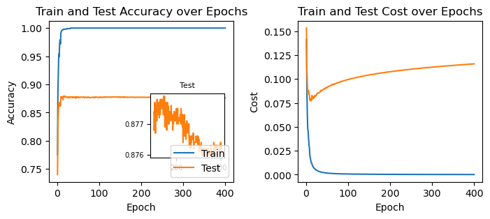

62.2 regularization

62.2.1 ridge regularization (L2)

net = ch3_code.NN2(layer_sizes=[784, 30, 10], rand_seed=3)
res2 = net.stochastic_gradient_descent(
     training_data=training_data[:1000],
     test_data=test_data,
     epochs=400,
     lmbda_L1=0.0,
     lmbda_L2=0.2,
     batch_size=10,
     eta=0.5,
     monitoring=True
     )

fig, ax = plt.subplots(1, 2, figsize=(8, 3))
fig.subplots_adjust(wspace=0.35)
ax[0].plot(res2["epoch"], res2["train_accuracy"], label="Train")
ax[0].plot(res2["epoch"], res2["test_accuracy"], label="Test")
ax[0].set_xlabel("Epoch")
ax[0].set_ylabel("Accuracy")
ax[0].set_title("Train and Test Accuracy over Epochs")
ax[0].legend()
axins = ax[0].inset_axes([0.55, 0.15, 0.4, 0.4])  # [x0, y0, width, height] in axes fraction
axins.plot(res2["epoch"][100:], res2["test_accuracy"][100:], color="tab:orange")
axins.set_title("Test", fontsize=8)
axins.tick_params(labelsize=7)

ax[1].plot(res2["epoch"], res2["train_cost"], label="Train Cost")
ax[1].plot(res2["epoch"], res2["test_cost"], label="Test Cost", color="tab:orange")
ax[1].set_xlabel("Epoch")
ax[1].set_ylabel("Cost")
ax[1].set_title("Train and Test Cost over Epochs");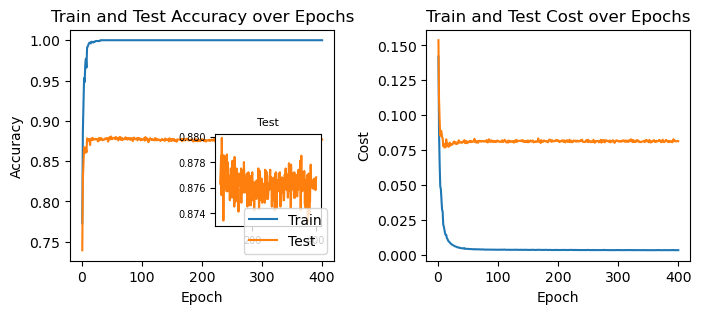

62.2.2 lasso regularization (L1)

net = ch3_code.NN2(layer_sizes=[784, 30, 10], rand_seed=3)
res3 = net.stochastic_gradient_descent(
     training_data=training_data[:1000],
     test_data=test_data,
     epochs=400,
     lmbda_L1=0.2,
     lmbda_L2=0.0,
     batch_size=10,
     eta=0.5,
     monitoring=True
     )

fig, ax = plt.subplots(1, 2, figsize=(8, 3))
fig.subplots_adjust(wspace=0.35)
ax[0].plot(res3["epoch"], res3["train_accuracy"], label="Train")
ax[0].plot(res3["epoch"], res3["test_accuracy"], label="Test")
ax[0].set_xlabel("Epoch")
ax[0].set_ylabel("Accuracy")
ax[0].set_title("Train and Test Accuracy over Epochs")
ax[0].legend()
axins = ax[0].inset_axes([0.55, 0.15, 0.4, 0.4])  # [x0, y0, width, height] in axes fraction
axins.plot(res3["epoch"][100:], res3["test_accuracy"][100:], color="tab:orange")
axins.set_title("Test", fontsize=8)
axins.tick_params(labelsize=7)

ax[1].plot(res3["epoch"], res3["train_cost"], label="Train Cost")
ax[1].plot(res3["epoch"], res3["test_cost"], label="Test Cost", color="tab:orange")
ax[1].set_xlabel("Epoch")
ax[1].set_ylabel("Cost")
ax[1].set_title("Train and Test Cost over Epochs");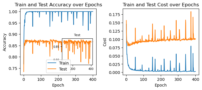

This is fascinating! We’re seeing a whole new kind of behavior. We now see sudden spikes in the accuracy and cost. What could be causing them?

I’m not sure, but it probably is because the L1 regularization pushes all weights to smaller absolute values with equal strength, regardless of their current value. This means that sometimes the weight updating may overshoot and cause the sign of the weight to flip. Add to that the fact that the L1 regularization tends to make many weights exactly zero. This is relavant, because a sudden change in the sign of the (few?) nonzero weights might cause a sudden change in the output of the network.

62.3 dropout

net = ch3_code.NN2(layer_sizes=[784, 30, 10], rand_seed=3)
res4 = net.stochastic_gradient_descent(
     training_data=training_data[:1000],
     test_data=test_data,
     epochs=100,
     lmbda_L1=0.0,
     lmbda_L2=0.2,
     batch_size=10,
     eta=0.5,
     dropout_prob=0.5,
     monitoring=True
     )