40 random forest
The motivation behind random forests is to avoid the weird regions in the feature space that a single decision tree might create. In the tutorial for classification with CART, we saw this: 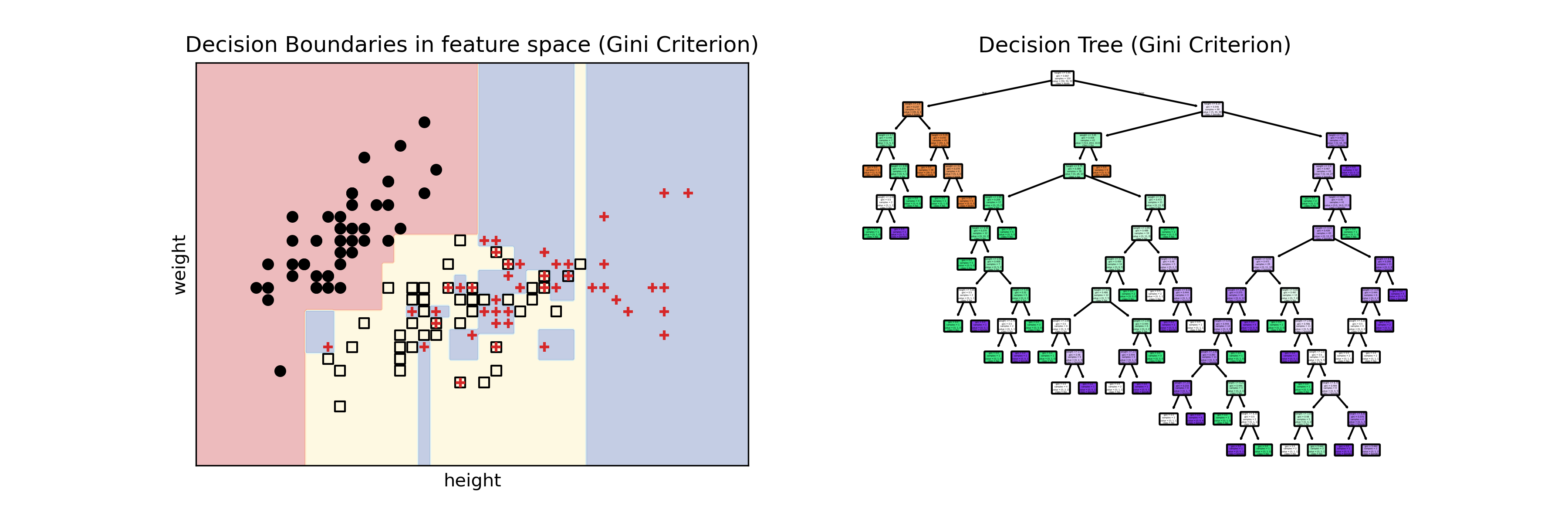
The small blue regions inside the yellow region are highly undesirable. The decision tree learned very well the data it was given, but it will probably not generalize well to new data points. Random forests solve this problem in three steps.
40.1 step 1: bootstrap sampling
Instead of running the decision tree algorithm once on the entire training set, we run it multiple times on different bootstrap samples of the training set. We already learned about bootstrap sampling in the empirical confidence interval tutorial. In a nutshell, if we have a data set with N data points, we create a bootstrap sample by sampling N data points with replacement from the original data set. This means that some data points will appear multiple times in the bootstrap sample, while others will not appear at all. We can choose how many bootstrap samples we want to create. The default used by sklearn’s RandomForestRegressor is 100 (this argument is called n_estimators).
What fraction of the dataset will a given bootstrap sample contain, on average? The probability of choosing a specific data point in one draw is 1/N. Therefore, the probability of not choosing that data point in one draw is 1 - 1/N. If we draw N times with replacement, the probability of never choosing that data point is
\left(1 - \frac{1}{N}\right)^N
As N becomes large…
\lim_{N \to \infty} \left(1 - \frac{1}{N}\right)^N = e^{-1} \approx 0.37.
This follows from the definition of the exponential function: e^x = \lim_{n \to \infty} \left(1 + \frac{x}{n}\right)^n, just set x = -1.
This means that, on average, a bootstrap sample will contain about 63% of the original data points (because about 37% of them will not be chosen at all).
40.2 step 2: random feature selection
When training each decision tree on a bootstrap sample, we also randomly select a subset of the features to consider for each split in the tree. For example, if we have 10 features in total, we might randomly select 3 of them to consider for each split. This further increases the diversity among the trees in the forest, which helps to reduce overfitting.
Why is this important? Imagine a dataset where feature number 1 is very strongly correlated with the target variable. In that case, most decision trees will likely use that feature for the top split, leading to similar trees and less diversity in the forest.
As a rule of thumb, we typically use the square root or the logarithm (base 2) of the total number of features as the number of features to consider for each split. The argument in sklearn’s RandomForestRegressor that controls this is called max_features, and its default value is 1.0. This means that if we don’t specify anything, it will use 100% of the features in each split, and we will not have “feature decorrelation”. In the documentation, search for max_features to find more details.
40.3 step 3: bagging
Finally, to make a prediction for a new data point, we pass it through each of the decision trees in the forest and average their predictions (for regression) or take a majority vote (for classification). This process is called “bagging” (short for bootstrap aggregating). By averaging the predictions of multiple trees, we can reduce the variance of the model and improve its generalization performance.
40.4 example: iris dataset
load iris dataset and prepare data
iris = load_iris()

# 1. Prepare Data (3 Inputs, 1 Output)
# columns: 0=SepalLen, 1=SepalWid, 2=PetalLen, 3=PetalWid
X_full = iris.data[:, [0, 1, 2]]  # 3 features
y_full = iris.data[:, 3]          # Target: Petal Width

# 2. Train Models
tree_model = DecisionTreeRegressor(random_state=42)
rf_model = RandomForestRegressor(n_estimators=100, random_state=42)

tree_model.fit(X_full, y_full)
rf_model.fit(X_full, y_full)

# 3. Compare Errors (The numerical proof)
print(f"Single Tree Score: {tree_model.score(X_full, y_full):.3f}")
print(f"Random Forest Score: {rf_model.score(X_full, y_full):.3f}")

# X = iris.data[:, [0, 1]]
# y = iris.data[:,[2]].flatten()
# iris.feature_names = ['height', 'weight', 'age']
Single Tree Score: 0.999
Random Forest Score: 0.991Show the code
from sklearn.model_selection import train_test_split

# 1. Split the data (80% for training, 20% for testing)
X_train, X_test, y_train, y_test = train_test_split(X_full, y_full, test_size=0.2, random_state=42)

# 2. Train on ONLY the training set
tree_model.fit(X_train, y_train)
rf_model.fit(X_train, y_train)

# 3. Test on the unseen data
print(f"Single Tree Test Score:   {tree_model.score(X_test, y_test):.3f}")
print(f"Random Forest Test Score: {rf_model.score(X_test, y_test):.3f}")
Single Tree Test Score: 0.845
Random Forest Test Score: 0.931