This equation states that the total variability in the response variable can be partitioned into two components: the variability explained by the regression model and the variability that is not explained by the model (the residuals).
In a more precise mathematical language, the equation states that:
\hat{y}_i are the predicted values from the regression model,
\bar{y} is the mean of the observed values,
n is the number of observations.
19.1 high-dimensional Pythagorean theorem
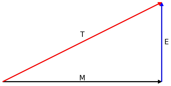
Why is this equation true? It’s easiest to understand this equation by thinking of it as a high-dimensional version of the Pythagorean theorem:
\lVert T \rVert ^2 = \lVert M \rVert ^2 + \lVert E \rVert ^2,
where:
T = y - \bar{y} is the total vector, the vector of deviations of the observed values from their mean;
M = \hat{y} - \bar{y} is the model vector, the vector of deviations of the predicted values from the mean of the observed values;
E = y - \hat{y} is the error vector, the vector of residuals, or deviations of the observed values from the predicted values.
I omitted the subscript i to emphasize that these are vectors, not scalars.
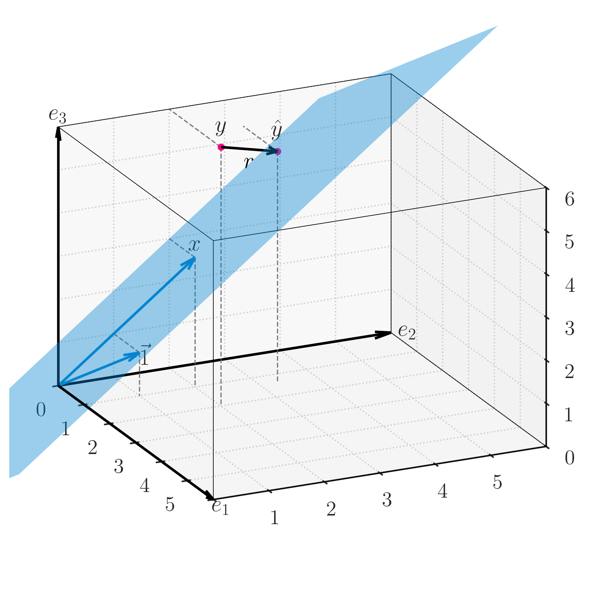
Make sure you understand the figure below, already presented in a previous chapter.
The vector r=E in black is the residual or error vector. It is orthogonal to the subspace spanned by the column vector of the design matrix, represented in this image by the blue plane.
The vector M is not shown, but it necessarily lies in the blue plane. How do we know that? Because the predicted values \hat{y} are a linear combination of the columns of the design matrix, and therefore \hat{y} lies in the column space of the design matrix. Since \bar{y} is a constant vector (a multiple of the vector of ones), it also lies in the column space of the design matrix. Therefore, M = \hat{y} - \bar{y} lies in the column space of the design matrix.
From the above, we can already conclude that E is orthogonal to M. These are the two legs of a right triangle. We now need a hypotenuse. The hypotenuse is the total vector T = y - \bar{y}, which is the sum of the other two vectors:
T = M + E.
This is easy to see by substituting the definitions of M and E:
T = y - \bar{y} = (\hat{y} - \bar{y}) + (y - \hat{y}) = M + E.