31 odds and log likelihood
31.1 the scenario
Imagine we are researchers studying a potential link between a specific mutated gene and a certain disease. We have collected data from a sample of 356 people.
Here’s our data:
| Has Disease | No Disease | |
|---|---|---|
| Has Mutated Gene | 23 | 117 |
| No Mutated Gene | 6 | 210 |
Our goal is to figure out how finding this mutated gene in a person should change our belief about whether they have the disease.
31.2 prior
The prior probability of someone having the disease is the chance of having the disease before we know anything about their gene status. We can calculate this from our data.
P(\text{Disease}) = \frac{\text{Number of people with the disease}}{\text{Total number of people}}
From our table: P(\text{Disease}) = \frac{23 + 6}{23 + 117 + 6 + 210} = \frac{29}{356} \approx 0.081
31.3 odds
Odds are a different way to express the same information. Odds compare the chance of an event happening to the chance of it not happening.
\text{Odds} = \frac{P(\text{event})}{P(\text{not event})}
In our case, “event” is having the disease. Because we have only two choices, the probability of not having the disease is simply 1 - P(\text{Disease}), therefore:
\text{Odds(Disease)} = \frac{P(\text{Disease})}{1 - P(\text{Disease})}
Plugging in the numbers:
\text{Odds(Disease)} = \frac{29/356}{1 - 29/356} \approx 0.0887 \approx \frac{1}{11}
This means that for every person with the disease, about 11 do not have it.
31.3.1 log odds
The log odds is simply the natural logarithm of the odds.
\text{Log Odds} = \ln\left(\frac{P}{1-P}\right)
We will see soon enough why this is useful. For now, let’s point out that:
- if the odds are 1 (meaning a 50/50 chance), the log odds is 0.
- if the odds are greater than 1 (more likely than not), the log odds is positive.
- if the odds are less than 1 (less likely than not), the log odds is negative.
- the log odds have a symmetric shape around p=1/2, see figure below.
For our example, the log odds of having the disease is:
\text{Log Odds(Disease)} = \ln(\text{Odds(Disease)}) = \ln(0.0887) \approx -2.42
visualize
fig, ax = plt.subplots(1, 2, figsize=(8, 6))

p = np.linspace(0, 1, 100)
odds = p / (1 - p)
ax[0].plot(p, odds, label="odds", color="tab:blue");
ax[0].axhline(1, ls="--", color="gray")
ax[0].set(ylabel="odds",
          xlabel="probability",
          title=r"f(p) = $\frac{p}{1-p}$",
          ylim=(-1, 10),
          xlim=(0, 1),
          xticks=[0,0.5,1]);
ax[0].annotate("more likely\nthan not", xy=(0.25, 1), xytext=(0.25, 3),
               ha="center", arrowprops=dict(arrowstyle="<-", color="gray"))
ax[0].annotate("less likely", xy=(0.7, 1), xytext=(0.7, -0.1),
               ha="center", arrowprops=dict(arrowstyle="<-", color="gray"))

ax[1].plot(p, np.log(odds), label="odds", color="tab:blue")
ax[1].axhline(0, ls="--", color="gray")
ax[1].yaxis.set_ticks_position('right')
ax[1].yaxis.set_label_position('right')
ax[1].set(ylabel="log odds",
          xlabel="probability",
          title=r"f(p) = log$\frac{p}{1-p}$",
          xlim=(0, 1),
          xticks=[0,0.5,1]);
ax[1].annotate("more likely\nthan not", xy=(0.25, 0), xytext=(0.25, 1),
               ha="center", arrowprops=dict(arrowstyle="<-", color="gray"))
ax[1].annotate("less likely", xy=(0.75, 0), xytext=(0.75, -1),
               ha="center", arrowprops=dict(arrowstyle="<-", color="gray"));
/var/folders/cn/m58l7p_j6j10_4c43j4pd8gw0000gq/T/ipykernel_10104/1581004145.py:5: RuntimeWarning: divide by zero encountered in divide
odds = p / (1 - p)
/var/folders/cn/m58l7p_j6j10_4c43j4pd8gw0000gq/T/ipykernel_10104/1581004145.py:19: RuntimeWarning: divide by zero encountered in log
ax[1].plot(p, np.log(odds), label="odds", color="tab:blue")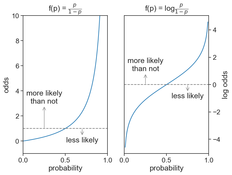
31.4 Bayes’ theorem in odds form
The standard form of Bayes’ theorem is:
P(H|E) = \frac{P(E|H) \cdot P(H)}{P(E)}. \tag{1}
In our example, the hypothesis H is “having the disease”, and the evidence E is detecting the mutated gene.
Let’s write Bayes’ theorem for the alternative hypothesis \neg H (“not having the disease”):
P(\neg H|E) = \frac{P(E|\neg H) \cdot P(\neg H)}{P(E)}. \tag{2}
The odds form of Bayes’ theorem is the ratio of these two equations:
\underbrace{\frac{P(H|E)}{P(\neg H|E)}}_ {\text{posterior odds}} = \underbrace{\frac{P(E|H)}{P(E|\neg H)}}_{\text{likelihood ratio}} \cdot \underbrace{\frac{P(H)}{P(\neg H)}}_{\text{prior odds}} \tag{3}
We already discussed the prior odds. The posterior odds represent the odds of having the desease after we have seen the evidence (the mutated gene). The new piece we need is the likelihood ratio.
31.5 likelihood ratio
The likelihood ratio (LR) tells us how much more likely we are to see the evidence if the hypothesis is true compared to if it is false.
\text{LR} = \frac{P(E|H)}{P(E|\neg H)}
We can compute this from our data:
- P(E|H): the probability of having the mutated gene given that the person has the disease. From the left column in our table, this is \frac{23}{23+6} \approx 0.793.
- P(E|\neg H): the probability of having the mutated gene given that the person does not have the disease. From the right column in our table, this is \frac{117}{117+210} \approx 0.358.
Finally:
\text{LR} = \frac{23/29}{117/327} \approx 2.22
The interpretation is that seeing the mutated gene is about 2.22 times more likely if the person has the disease than if they do not.
31.6 log likelihood ratio
Here too, taking the logarithm transforms a quantity between 0 and infinity into a number between negative infinity and positive infinity. The log likelihood ratio is: \text{Log-LR} = \ln(\text{LR}) = \ln(2.22) \approx 0.797
The fact that this is a positive number says that seeing the mutated gene increases our belief that the person has the disease.
31.7 Bayes’ theorem in log odds form
Taking the logarith of Eq. (3) gives us the log odds form of Bayes’ theorem:
\underbrace{\ln\left(\frac{P(H|E)}{P(\neg H|E)}\right)}_{\text{posterior log odds}} = \underbrace{\ln\left(\frac{P(E|H)}{P(E|\neg H)}\right)}_{\text{log-likelihood ratio}} + \underbrace{\ln\left(\frac{P(H)}{P(\neg H)}\right)}_{\text{prior log odds}} \tag{4}
Plugging in our numbers, we can see how our belief about the person having the disease changes after seeing the evidence (the mutated gene).
\begin{align*} \text{Posterior Log Odds} &= \text{Log-LR} + \text{Prior Log Odds} \\ &= 0.797 + (-2.42) \\ &\approx -1.623 \end{align*}
From the posterior log odds, we can get back to the posterior odds by exponentiating:
\text{Posterior Odds} = e^{\text{Posterior Log Odds}} = e^{-1.623} \approx 0.197
Finally, we can convert the posterior odds back to a probability: P(H|E) = \frac{\text{Posterior Odds}}{1 + \text{Posterior Odds}} = \frac{0.197}{1 + 0.197} \approx 0.164 This means that after seeing the mutated gene, our estimate of the probability that the person has the disease has increased from about 8.1% to about 16.4%.