37 SVD for regression
This tutorial is partly based on the following sources:
- Understanding Linear Regression using the Singular Value Decomposition by Thalles Silva.
- Brunton and Kutz’s book, Data-Driven Science and Engineering, subsection 1.4 called “Pseudo-inverse, least-squares, and regression”.
37.1 the problem with Ordinary Least Squares
Let’s say I want to predict the weight of a person based on their height. I have the following data:
| Height (cm) | Weight (kg) |
|---|---|
| 150 | 53 |
| 160 | 65 |
| 170 | 68 |
| 180 | 82 |
| 190 | 88 |
visualize data
Text(0, 0.5, 'Weight (kg)')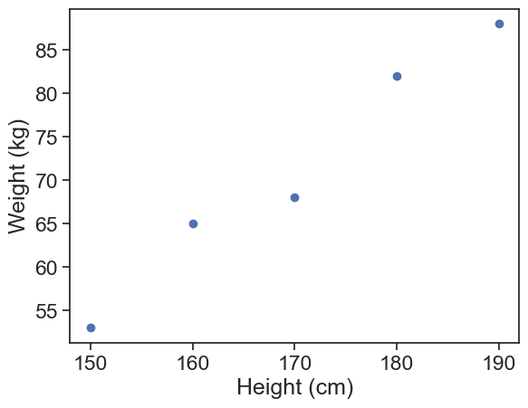
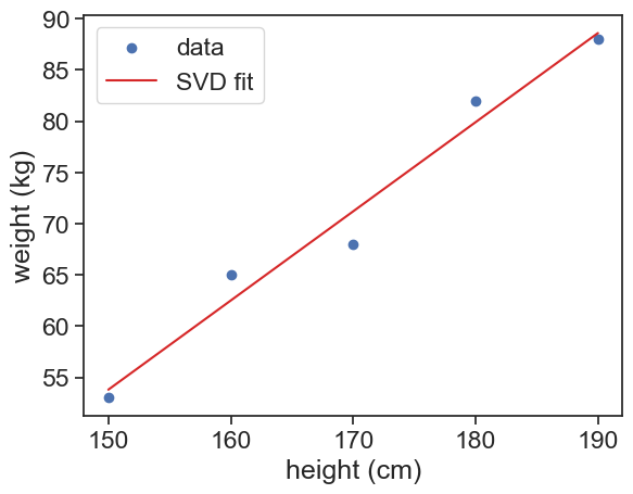
I can try to predict the weight using a linear model:
\text{weight} = \beta_0 + \beta_1 \cdot \text{height}. \tag{1}
In a general form, we can write this as:
X\beta = y, \tag{2}
where X is the design matrix, \beta is the vector of coefficients, and y is the vector of outputs (weights). This problem probably has no exact solution for \beta, because the design matrix X is not square (there are more data points than parameters). So we want to find the best approximation \hat{\beta} that minimizes the error:
\hat{\beta} = \arg\min_\beta \|y - X\beta\|^2. \tag{3}
We know how to solve this, we use the equation we derived in the chapter “the geometry of regression”:
\hat{\beta} = (X^TX)^{-1}X^Ty, \tag{4}
For a linear model, the design matrix is:
X = \begin{bmatrix} | & | \\ \mathbf{1} & h\\ | & | \end{bmatrix} = \begin{bmatrix} 1 & 150 \\ 1 & 160 \\ 1 & 170 \\ 1 & 180 \\ 1 & 190 \end{bmatrix} . \tag{5}
What does the matrix X^T X look like?
\begin{align*} X^TX &= \begin{bmatrix} - & \mathbf{1}^T & - \\ - & h^T & - \end{bmatrix} \begin{bmatrix} | & | \\ \mathbf{1} & h\\ | & | \end{bmatrix}\\ &= \begin{bmatrix} \mathbf{1}^T\mathbf{1} & \mathbf{1}^Th \\ h^T\mathbf{1} & h^Th \end{bmatrix}\\ &= \begin{bmatrix} 5 & 850 \\ 850 & 153000 \end{bmatrix} \tag{6} \end{align*}
There’s no problem inverting this matrix, so we can find the coefficient estimates \hat{\beta} using the formula above.
Suppose now that we have a new predictor, the height of the person in inches. The design matrix now looks like this:
X = \begin{bmatrix} | & | & | \\ \mathbf{1} & h_{cm} & h_{inch}\\ | & | & | \end{bmatrix} \tag{7}
Obviously, the columns h_{cm} and h_{inch} are linearly dependent (h_{cm}=ah_{inch}). This means that the matrix X^TX also has linearly dependent columns:
\begin{align*} X^TX &= \begin{bmatrix} - & \mathbf{1}^T & - \\ - & h_{cm}^T & - \\ - & h_{inch}^T & - \end{bmatrix} \begin{bmatrix} | & | & | \\ \mathbf{1} & h_{cm} & h_{inch}\\ | & | & | \end{bmatrix} \\ &= \begin{bmatrix} \mathbf{1}^T\mathbf{1} & \mathbf{1}^Th_{cm} & \mathbf{1}^Th_{inch} \\ h_{cm}^T\mathbf{1} & h_{cm}^Th_{cm} & h_{cm}^Th_{inch} \\ h_{inch}^T\mathbf{1} & h_{inch}^Th_{cm} & h_{inch}^Th_{inch} \end{bmatrix} \tag{8} \end{align*}
Using the fact that h_{cm}=ah_{inch}, we can see that the second and third columns are linearly dependent. This means that the matrix X^TX is not invertible, and we cannot use the formula above to find the coefficient estimates \hat{\beta}. What now?
This is an extreme case, but problems similar to this can happen in real life. For example, if we have two predictors that are highly correlated, the matrix X^TX will be close to singular (not invertible). In this case, the coefficients \beta will be very sensitive to small changes in the data.
37.2 SVD to the rescue
Let’s use Singular Value Decomposition (SVD) to find the coefficients \beta. SVD is a powerful technique that can handle multicollinearity and other issues in the data.
The SVD of a matrix X is given by:
X = U\Sigma V^T, \tag{9}
where U and V are orthogonal matrices and \Sigma is a diagonal matrix with singular values on the diagonal.
We can plug the SVD of X into the least squares problem, which is to find the \hat{\beta} that best satisfies X\hat{\beta} = \hat{y}:
U\Sigma V^T\hat{\beta} = \hat{y}. \tag{10}
We define now the Moore-Penrose pseudo-inverse of X, which is given by:
X^+ = V\Sigma^+U^T, \tag{11}
where \Sigma^+ is obtained by taking the reciprocal of the non-zero singular values in \Sigma and transposing the resulting matrix.
This pseudo-inverse has the following properties:
X^+X = I. This means that X^+ is a left-inverse of X.
XX^+ is a projection matrix onto the column space of X. In other words, left-multiplying XX^+ to any vector gives the projection of that vector onto the column space of X. In particular, XX^+y = \hat{y}.
This is very similar to the property we used in the chapter “the geometry of regression”, where we had P_Xy = \hat{y}, with P_X being the projection matrix onto the column space of X. There, we found that
\hat{\beta} = (X^TX)^{-1}X^Ty,
Left-multiplying both sides by X gives: X\hat{\beta} = X(X^TX)^{-1}X^Ty = P_Xy = \hat{y}. So we found that in the OLS case, X(X^TX)^{-1}X^T is the projection matrix onto the column space of X. Here, we have a more general result that works even when X^TX is not invertible: XX^+ is the projection matrix onto the column space of X.
We left-multiply Eq. (10) by X^+, and also substitute \hat{y}=XX^+y as we just saw:
\begin{align*} X^+ (U\Sigma V^T\hat{\beta}) &= X^+XX^+y\\ (V\Sigma^+U^T)(U\Sigma V^T)\hat{\beta} &= X^+y \tag{12} \end{align*}
The term (V\Sigma^+U^T)(U\Sigma V^T) simplifies to the identity matrix, so we have:
\hat{\beta} = X^+y = V\Sigma^+U^Ty. \tag{13}
This is the formula we will use to find the coefficients \hat{\beta} using SVD. This formula works even when X^TX is not invertible, and it is more stable than the OLS formula.
37.3 in practice
Let’s go back to the problematic example with height in cm and inches. We can use the SVD to find the coefficients \hat{\beta}.
# design matrix with intercept, height in cm and height in inches
conversion_factor = 2.54
X = np.vstack([np.ones(len(h)), h, h/conversion_factor]).T
# compute SVD of X
U, S, VT = np.linalg.svd(X, full_matrices=False)
Sigma = np.diag(S)
V = VT.T
# compute coefficients using SVD
y = w
Sigma_plus = np.zeros(Sigma.T.shape)
for i in range(len(S)):
    if S[i] > 1e-10:  # avoid division by zero
        Sigma_plus[i, i] = 1 / S[i]
X_plus = V @ Sigma_plus @ U.T
beta_hat = X_plus @ y
# make predictions
y_hat = X @ beta_hat