2 weight data
Now that we have height data covered, it’s time we deal with weight data.
Yes, I am VERY WELL AWARE that weight is a force, and it is not measured in kg. Nevertheless, I will use the word weight in the colloquial sense, and for all purposes it is a synonym for mass.
This analysis is based on the CDC Growth Charts Data Files. From there I downloaded a csv for the weight of boys and girls, from age 2 to 20.
For each sex and age, the csv contains three important columns for us:
- M: median
- S: generalized coefficient of variation
- L: Box-Cox power
These three variables can be combined to give the weight W at a given Z-score (number of standard deviations from the mean):
W = M \left(1 + L S Z\right)^{1/L} \tag{1}
The website contains a different formula for the case L=0, but in our data set L is never zero.
It will be useful in a little while to know the inverse of Eq. (1), which is
Z = \frac{(W/M)^L - 1}{L S}. \tag{1b}
The formulas above indicate that we’re using the Box-Cox distribution (also called power-normal distribution), and they will help us compute the probability density function (pdf) for weight.
Given that the pdf of a z-scored variable is f_z(Z) = \frac{1}{\sqrt{2 \pi}} e^{-Z^2/2}, \tag{2}
we need to change variables from Z to W. To do that, we will use
f_w(W)dW = f_z(Z)dZ. \tag{3}
The rationale behind this is that the probability (area) of being in a small interval is the same, whether we measure it in terms of W or Z. See more here: Function of random variables and change of variables in the probability density function. Solving Eq. (3) for f_w(W), we get
f_w(W) = f_z(Z) \left|\frac{dZ}{dW}\right| = f_z(Z) \left|\frac{dW}{dZ}\right|^{-1}. \tag{4}
Using Eq. (1), the derivative of W with respect to Z is
\begin{align*} \frac{dW}{dZ} &= MS\left(1+LSZ\right)^{\frac{1}{L}-1}\\ &= \underbrace{M\left(1+LSZ\right)^{\frac{1}{L}}}_{=W \text{ according to Eq. (1)}}S\left(1+LSZ\right)^{-1} \\ &= WS\frac{1}{1+LSZ} \\ &= WS\frac{1}{\bcancel{1}+\cancel{LS}\frac{(W/M)^L - \bcancel{1}}{\cancel{L S}}} \\ &= WS\frac{1}{(W/M)^L} \\ & = W^{1-L} M^L S \tag{5} \end{align*}
Putting everything together [remember that we need the reciprocal of the result in Eq. (5)], we get
\begin{align*} f_w(W) &= f_z(Z) \frac{W^{L-1}}{M^L S} \\ &= \frac{1}{\sqrt{2 \pi}} e^{-Z^2/2} \frac{W^{L-1}}{M^L S} \tag{6} \end{align*}
Of course, we could have substituted Z from Eq. (1b) into Eq. (6) to get a formula that depends only on W, it would be too messy. Later on, we will compute f_w(W) numerically, so we will not need to do that.
2.1 example
Let’s see the weight probability density for boys at age 10 and 15.
load weight data and compute pdf
weight_list = np.arange(10, 130, 0.1)
def power_normal_pdf(w, age, sex):
    """
    Calculates the PDF of the Power Normal distribution from the derived formula.
    This function correctly handles negative L values.
    """
    # This function is only valid for w > 0
    w = np.asarray(w)
    pdf = np.full(w.shape, np.nan)
    positive_w = w[w > 0]
    df = pd.read_csv('../archive/data/weight/wtage.csv')
    agemos = age * 12 + 0.5
    df = df[(df['Agemos'] == agemos) & (df['Sex'] == sex)]
    L = df['L'].values[0]
    M = df['M'].values[0]
    S = df['S'].values[0]

    # Calculate the z-score
    z = ((positive_w / M)**L - 1) / (L * S)

    # Calculate the two main parts of the formula
    pre_factor = positive_w**(L - 1) / (S * M**L * np.sqrt(2 * np.pi))
    exp_term = np.exp(-0.5 * z**2)

    # Store the results only for the valid (positive w) indices
    pdf[w > 0] = pre_factor * exp_term
    return pdf

pdf_boys10 = power_normal_pdf(weight_list, 10, 1)
pdf_boys15 = power_normal_pdf(weight_list, 15, 1)
plot
fig, ax = plt.subplots(figsize=(8, 6))
ax.plot(weight_list, pdf_boys10, color='tab:blue', lw=2, alpha=0.5, label='10 years')
ax.plot(weight_list, pdf_boys15, color='tab:blue', lw=2, label='15 years')
ax.set(xlabel='weight (kg)',
       ylabel='pdf',
       title="weight distribution for boys")
ax.legend(loc="upper right", frameon=False)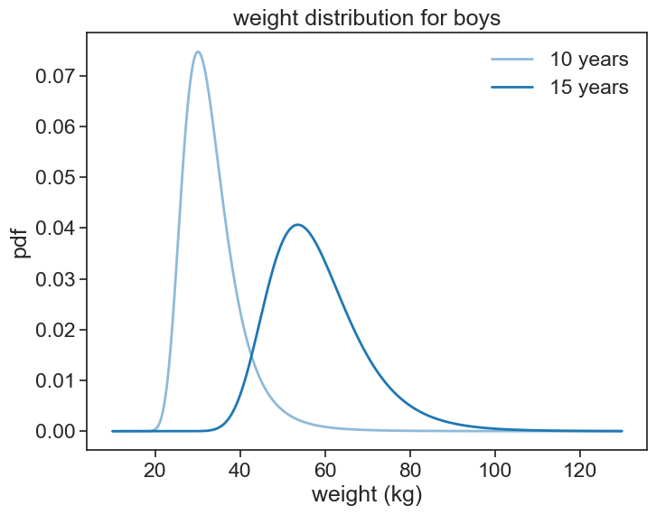
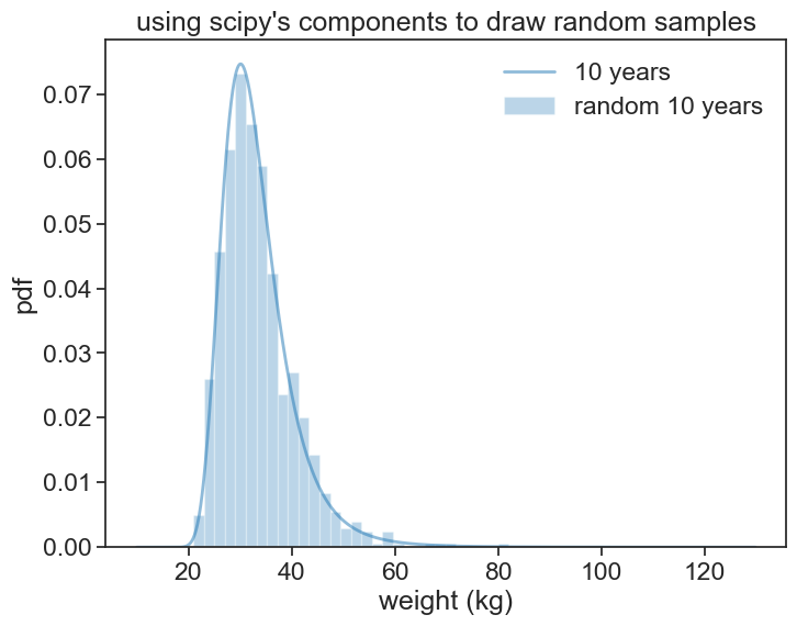
In future chapters, when we want to talk about weight, it will be more convenient to leverage scipy’s capabilities, both to compute the pdf and to generate random samples.
leveraging scipy.stats
def scipy_power_normal_pdf(w, age, sex):

    # Load LMS parameters from the CSV file
    df = pd.read_csv('../archive/data/weight/wtage.csv')
    agemos = age * 12 + 0.5
    df = df[(df['Agemos'] == agemos) & (df['Sex'] == sex)]
    L = df['L'].values[0]
    M = df['M'].values[0]
    S = df['S'].values[0]

    # 1. Transform weight (w) to the standard normal z-score
    z = ((w / M)**L - 1) / (L * S)

    # 2. Calculate the derivative of the transformation (dz/dw)
    # This is the Jacobian factor for the change of variables
    dz_dw = (w**(L - 1)) / (S * M**L)

    # 3. Apply the change of variables formula: pdf(w) = pdf(z) * |dz/dw|
    pdf = stats.norm.pdf(z) * dz_dw

    return pdf

def scipy_power_normal_draw_random(N, age, sex):
    # Load LMS parameters from the CSV file
    df = pd.read_csv('../archive/data/weight/wtage.csv')
    agemos = age * 12 + 0.5
    df = df[(df['Agemos'] == agemos) & (df['Sex'] == sex)]
    L = df['L'].values[0]
    M = df['M'].values[0]
    S = df['S'].values[0]

    # draw random z from standard normal distribution
    z = np.random.normal(0, 1, N)
    # transform z to w
    w = M * (1 + L * S * z)**(1 / L)

    return w

# Calculate the PDFs for 10 and 15-year-old boys using the SciPy-based function
scipy_pdf_boys10 = scipy_power_normal_pdf(weight_list, 10, 1)
draw10 = scipy_power_normal_draw_random(1000, 10, 1)
scipy_pdf_boys15 = scipy_power_normal_pdf(weight_list, 15, 1)
plot
fig, ax = plt.subplots(figsize=(8, 6))
ax.plot(weight_list, pdf_boys10, color='tab:blue', lw=2, alpha=0.5, label='10 years')
# histogram of draw10
ax.hist(draw10, bins=30, density=True, color='tab:blue', alpha=0.3, label='random 10 years')
# ax.plot(weight_list, scipy_pdf_boys10, color='tab:blue', ls=":", label='scipy 10')
ax.set(xlabel='weight (kg)',
       ylabel='pdf',
       title="using scipy's components to draw random samples")
ax.legend(loc="upper right", frameon=False)