59 Nielsen’s NNDL, ch.1
In this notebook I’ll follow Michael Nielsen’s book Neural Networks and Deep Learning. I’ll make comments if I feel they add something to the original test. If you don’t understand everything here, don’t worry, you’re not supposed to, just refer to the original book if you’re interested in the details.
59.1 loading the data
In the Common Visual Data Foundation’s Github, I found the URLs for the MNIST dataset. I will load the data directly into memory using these URLs, without saving them to disk.
define function to load MNIST from web
def load_mnist_from_web():
    urls = {
        "train_img": "https://storage.googleapis.com/cvdf-datasets/mnist/train-images-idx3-ubyte.gz",
        "train_lbl": "https://storage.googleapis.com/cvdf-datasets/mnist/train-labels-idx1-ubyte.gz",
        "test_img": "https://storage.googleapis.com/cvdf-datasets/mnist/t10k-images-idx3-ubyte.gz",
        "test_lbl": "https://storage.googleapis.com/cvdf-datasets/mnist/t10k-labels-idx1-ubyte.gz"
    }

    data_results = {}

    for key, url in urls.items():
        print(f"Fetching {key}...")
        response = requests.get(url)
        response.raise_for_status()

        # Wrap the content in BytesIO and decompress in memory
        with gzip.GzipFile(fileobj=io.BytesIO(response.content)) as f:
            if "img" in key:
                # Images: offset 16
                data_results[key] = np.frombuffer(f.read(), np.uint8, offset=16)
            else:
                # Labels: offset 8
                data_results[key] = np.frombuffer(f.read(), np.uint8, offset=8)

    # Re-format to Nielsen's expected structure
    def vectorized_result(j):
        e = np.zeros((10, 1))
        e[j] = 1.0
        return e

    training_inputs = [np.reshape(x, (784, 1)) / 255.0 for x in data_results["train_img"].reshape(-1, 784)]
    training_results = [vectorized_result(y) for y in data_results["train_lbl"]]
    training_data = list(zip(training_inputs, training_results))

    test_inputs = [np.reshape(x, (784, 1)) / 255.0 for x in data_results["test_img"].reshape(-1, 784)]
    test_data = list(zip(test_inputs, data_results["test_lbl"]))

    return training_data, test_data
load MNIST data into memory
Fetching train_img...
Fetching train_lbl...
Fetching test_img...
Fetching test_lbl...
Loaded 60000 training samples directly into memory.
Let’s see a few of the images in the training set:
see some sample images
fig, ax = plt.subplots(5, 5, figsize=(5, 5))
ax = ax.flatten()
for i in range(25):
    ax[i].imshow(training_data[i][0].reshape(28, 28), cmap='gray')
    label = np.argmax(training_data[i][1])
    ax[i].text(0.97, 0.97, f"{label}", transform=ax[i].transAxes,
         horizontalalignment='right', verticalalignment='top',
         fontweight="bold", color="xkcd:goldenrod")
    ax[i].axis('off')
fig.suptitle("Sample MNIST Training Images", fontsize=16);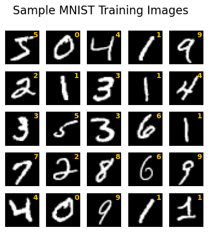
The training set has one-hot encoded labels, while the test set has integer labels. That’s perfect for our purposes!
Show the code
fig, ax = plt.subplots(1, 2, figsize=(8, 3))
ax[0].imshow(training_data[0][0].reshape(28, 28), cmap='gray')
ax[0].text(-0.05, 0.5, "label:\n" + f"{training_data[0][1]}", transform=ax[0].transAxes,
         horizontalalignment='right', verticalalignment='center',)
ax[0].set_title("Training Sample")

ax[1].imshow(test_data[0][0].reshape(28, 28), cmap='gray')
ax[1].text(-0.05, 0.5, "label:\n" + f"{test_data[0][1]}", transform=ax[1].transAxes,
         horizontalalignment='right', verticalalignment='center',)
ax[1].set_title("Test Sample")
ax[0].axis('off')
ax[1].axis('off');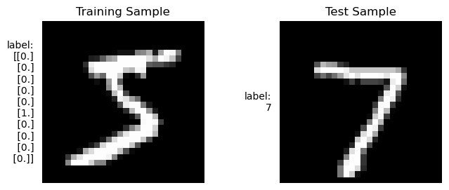
59.2 exercise A
Sigmoid neurons simulating perceptrons, part I
Suppose we take all the weights and biases in a network of perceptrons, and multiply them by a positive constant, c>0. Show that the behaviour of the network doesn’t change.
\text{perceptron output} = \begin{cases} 1 & \text{if } z > 0 \\ 0 & \text{otherwise} \end{cases},
where z=\sum_{i=1}^{n} w_i x_i + b.
We start with the expression z=w_i x_i + b. Multiplying all weights and biases by a positive constant c gives us c w_i x_i + c b. We can factor out the constant to get cz. Since c is positive, the sign of the expression remains unchanged. Therefore, the output of the perceptron will still be 1 if cz > 0 and 0 otherwise, meaning the behavior of the network does not change.
59.3 exercise B
Sigmoid neurons simulating perceptrons, part II
Suppose we have the same setup as the last problem — a network of perceptrons. Suppose also that the overall input to the network of perceptrons has been chosen. We won’t need the actual input value, we just need the input to have been fixed. Suppose the weights and biases are such that w\cdot x+b\neq 0 for the input x to any particular perceptron in the network. Now replace all the perceptrons in the network by sigmoid neurons, and multiply the weights and biases by a positive constant c>0. Show that in the limit as c\rightarrow \infty the behaviour of this network of sigmoid neurons is exactly the same as the network of perceptrons. How can this fail when w\cdot x+b= 0 for one of the perceptrons?
Sigmoid function
\sigma(z) = \frac{1}{1 + e^{-z}}
Once more, multiplying the weights and biases by c gives us cz as the argument to the sigmoid function:
\sigma(cz) = \frac{1}{1 + e^{-cz}} = \frac{1}{1 + \left(e^{-z}\right)^c}
The factor e^{-z}<1 if z is positive, and e^{-z}>1 if z is negative. Taking c to infinity raises e^{-z} to the power of infinity, which gives us 0 if z is positive and infinity if z is negative. Therefore, \sigma(cz) approaches 1 if z is positive and 0 if z is negative, which is the same behavior as a perceptron. See the graph below.
sigmoid function with different steepness
fig, ax = plt.subplots(1, 1, figsize=(5, 3))
z = np.linspace(-2, 2, 1001)
sigma = lambda z: 1 / (1 + np.exp(-z))
c_list = [1, 5, 20, 100]
colors = plt.cm.Blues(np.linspace(0.3, 1.0, len(c_list)))
for c, color in zip(c_list, colors):
    ax.plot(z, sigma(c * z), color=color, label=f"c={c}")
ax.legend(loc="upper left", frameon=False)
ax.set(xlabel="z",
       title="sigmoid with different steepness (c)");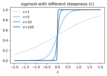
However, if w\cdot x + b = 0, then z=0 and \sigma(cz) = \sigma(0) = 0.5 for all values of c, which does not match the behavior of a perceptron, which would output 0 in this case.
59.4 exercise C
bitwise representation
There is a way of determining the bitwise representation of a digit by adding an extra layer to the three-layer network above. The extra layer converts the output from the previous layer into a binary representation, as illustrated in the figure below. Find a set of weights and biases for the new output layer. Assume that the first 3 layers of neurons are such that the correct output in the third layer (i.e., the old output layer) has activation at least 0.99, and incorrect outputs have activation less than 0.01.
Instead of thinking what are the weights and biases for each of the 4 output neurons, we can think of the weights and biases for each of the 10 neurons in the previous layer. We do that by writing the binary representation of the output digit, for example:
0 = 0000
1 = 0001
2 = 0010
3 = 0011
4 = 0100
5 = 0101
6 = 0110
7 = 0111
8 = 1000
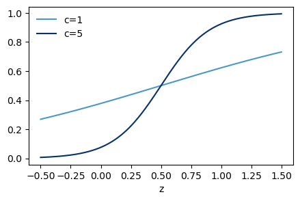
9 = 1001The first column corresponds to the weights for the first output neuron, the second column corresponds to the weights for the second output neuron, and so on. In order to get activation for z=1 and no activation for z=0, we can shift the sigmoid function to the right by setting the bias to -0.5. This way, if the input is 1, we get z=1-0.5=0.5 which gives us an activation of \sigma(0.5) \approx 0.62, and if the input is 0, we get z=0-0.5=-0.5 which gives us an activation of \sigma(-0.5) \approx 0.38. This is enought to make it work, but the constrast between “on” and “off” is not very high. We can increase the contrast by multiplying the weights and biases by a positive constant c, as we saw in the previous exercises. For example, if we set c=10, then for an input of 1 we get z=10*1-10*0.5=5 which gives us an activation of \sigma(5) \approx 0.993, and for an input of 0 we get z=10*0-10*0.5=-5 which gives us an activation of \sigma(-5) \approx 0.007.
sigmoid function
fig, ax = plt.subplots(1, 1, figsize=(5, 3))
z = np.linspace(-0.5, 1.5, 1001)
sigma = lambda z: 1 / (1 + np.exp(-z))
c_list = [1, 5]
colors = plt.cm.Blues(np.linspace(0.6, 1.0, len(c_list)))
for c, color in zip(c_list, colors):
    ax.plot(z, sigma(c * (z-0.5)), color=color, label=f"c={c}")
ax.legend(loc="upper left", frameon=False)
ax.set(xlabel="z",
    #    title="sigmoid with different steepness (c)"
       );
Show the code
# essential for Quarto static HTML embedding
rc('animation', html='jshtml')

def sigma(x):
    return 1 / (1 + np.exp(-x))

N = 10
w = np.array([[int(c) for c in f"{num:04b}"[::-1]] for num in range(N)])
b = -0.5 * np.ones(4)
ms = 20

fig, ax = plt.subplots(1, 1, figsize=(5, 5))

def update(frame):
    ax.clear()
    neuron_on = frame

    # input state
    x = np.zeros(N) + 0.01
    x[neuron_on] = 0.99

    # calculation
    z = np.dot(w.T, x) + b
    output = sigma(10 * z)

    # draw weights
    for i, row in enumerate(w):
        color = "xkcd:vermillion" if i == neuron_on else "gray"
        for j, val in enumerate(row):
            alpha = 1.0 if val == 1 else 0.2
            ax.plot([0, 1], [N - i, (4 - j) + 3], color=color, lw=2, alpha=alpha)

    # draw input neurons (LHS)
    for i in range(N):
        mfc = "xkcd:vermillion" if x[i] > 0.5 else "white"
        ax.plot([0], [N - i], ls='None', marker='o', mfc=mfc,
                mec="xkcd:vermillion", markersize=ms)
        ax.text(-0.1, N - i, f"{i}", va='center', ha='right', fontsize=14)

    # draw output neurons (RHS)
    for i in range(4):
        shade = str(1 - output[i]) # grayscale string for mfc, black = on
        ax.plot([1], [(4 - i) + 3], ls='None', marker='o', mfc=shade,
                mec="black", markersize=ms)
        ax.text(1 + 0.1, (4 - i) + 3, f"{2**i}", va='center', ha='left', fontsize=14)

    ax.text(0, 0, "old output layer", va="top", ha="center", fontsize=14)
    ax.text(1, 0, "new output layer", va="top", ha="center", fontsize=14)

    ax.set(xlim=(-0.5, 1.5), ylim=(0, N + 1), xticks=[], yticks=[])
    ax.set_title(f"Active Neuron: {neuron_on}")
    ax.axis('off')

# create animation: 10 frames (0 through 9)
anim = FuncAnimation(fig, update, frames=range(N), interval=500)

plt.close(fig)  # prevents the static plot from being captured
anim # calling 'anim' displays the JS player59.5 exercise D
Indeed, there’s even a sense in which gradient descent is the optimal strategy for searching for a minimum. Let’s suppose that we’re trying to make a move \Delta v in position so as to decrease C as much as possible. This is equivalent to minimizing \Delta C≈\nabla C\cdot\Delta v. We’ll constrain the size of the move so that \Vert \Delta v\Vert=\epsilon for some small fixed \epsilon>0. In other words, we want a move that is a small step of a fixed size, and we’re trying to find the movement direction which decreases C as much as possible. It can be proved that the choice of \Delta v which minimizes \nabla C\cdot\Delta v is \Delta v=−\eta\nabla C, where \eta=\epsilon/\Vert\nabla C\Vert is determined by the size constraint \Vert\Delta v\Vert=\epsilon. So gradient descent can be viewed as a way of taking small steps in the direction which does the most to immediately decrease C.
gradient descent as an optimal strategy
Prove the assertion of the last paragraph. Hint: If you’re not already familiar with the Cauchy-Schwarz inequality, you may find it helpful to familiarize yourself with it.
The Cauchy-Schwarz inequality states that for any vectors a and b, we have: |a \cdot b| \leq \Vert a \Vert \Vert b \Vert
with equality if and only if a and b are linearly dependent. In our case, we want to minimize \nabla C \cdot \Delta v subject to \Vert \Delta v \Vert = \epsilon. We can rewrite this as:
\nabla C \cdot \Delta v = \Vert \nabla C \Vert \Vert \Delta v \Vert \cos(\theta)
where \theta is the angle between \nabla C and \Delta v. To minimize this expression, we want the smallest value of \cos(\theta), which is -1 when \theta = \pi, meaning that \Delta v is in the opposite direction of \nabla C. Therefore, we have: \Delta v = -\eta \nabla C where \eta is a positive constant that ensures \Vert \Delta v \Vert = \epsilon. We can find \eta by solving for it in the constraint: \Vert \Delta v \Vert = \Vert -\eta \nabla C \Vert = \eta \Vert \nabla C \Vert = \epsilon which gives us: \eta = \frac{\epsilon}{\Vert \nabla C \Vert}, therefore \Delta v = -\frac{\epsilon}{\Vert \nabla C \Vert} \nabla C.
The step in the parameter space is in the opposite direction of the unitary vector of the gradient, and its size is \epsilon, which is the maximum allowed step size. This shows that gradient descent is the optimal strategy for searching for a minimum under the given constraints.
59.6 exercise E
geometric interpretation of gradient descent
I explained gradient descent when C is a function of two variables, and when it’s a function of more than two variables. What happens when C is a function of just one variable? Can you provide a geometric interpretation of what gradient descent is doing in the one-dimensional case?
The gradient descent algorithm in the one-dimensional case is essentially performing a simple iterative process to find the local minimum of a function. In this case, the “gradient” is just the derivative of the function with respect to the variable.
59.7 exercise F
pros and cons of online learning
An extreme version of gradient descent is to use a mini-batch size of just 1. That is, given a training input, x, we update our weights and biases according to the rules w_k\rightarrow w'_k=w_k−\eta \partial C_x/\partial w_k and b_l\rightarrow b'_l=b_l−\eta\partial C_x/\partial b_l. Then we choose another training input, and update the weights and biases again. And so on, repeatedly. This procedure is known as online, on-line, or incremental learning. In online learning, a neural network learns from just one training input at a time (just as human beings do). Name one advantage and one disadvantage of online learning, compared to stochastic gradient descent with a mini-batch size of, say, 20.
Advantage: We have the hope of learning which weights and biases in our network are most associated with a given training input, which can be useful for interpretability and understanding the model’s behavior.
Disadvantage: The path in the parameter space will by so much noisier than with a mini-batch size of 20, which can make it harder to converge to a good minimum.
59.8 exercise G
Equation 22:
a'=\sigma(w\cdot a + b)
Equation 4:
\frac{1}{1+\exp\left(-\sum_{j} w_j x_j - b\right)}
equivalent results
Write out Equation (22) in component form, and verify that it gives the same result as the rule (4) for computing the output of a sigmoid neuron.
a' are the activation values of the layer on the right, and a are the activation values of the layer on the left. Let’s call a=x
z = w\cdot a + b = w\cdot x + b \\
Let’s write the vector z with explicit indices:
\begin{align*} z_i &= (w\cdot x)_i + b_i \\ &= \left(\sum_j w_{ij}\cdot x_j\right) + b_i \end{align*}
Show the code
fig, ax = plt.subplots(figsize=(5, 5))

layer_left = 7
layer_right = 4
ms = 12
for i in range(layer_left):
    for j in range(layer_right):
        if j == 1:
            color = "xkcd:cerulean"
            alpha = 1.0
        else:
            alpha = 0.5
            color = "gray"
        ax.plot([0, 1], [(layer_left - i)/layer_left, (layer_right - j + 1.5)/layer_left],
                color=color, lw=2, alpha=alpha)


for i in range(layer_left):
    ax.plot([0], [(layer_left - i)/layer_left], ls='None', marker='o', mfc="xkcd:vermillion",
            mec="gray", markersize=ms, alpha=1.0)
    ax.text(-0.1, (layer_left - i)/layer_left, fr"$x_{i}$",
                va='center', ha='right', fontsize=12, color="gray")

for i in range(layer_right):
    if i==1: color = "xkcd:goldenrod"
    else: color = "white"
    ax.plot([1], [(layer_right - i + 1.5)/layer_left], ls='None', marker='o', mfc=color,
            mec="gray", markersize=ms)
    ax.text(1.1, (layer_right - i + 1.5)/layer_left, fr"$a_{i}=\sigma(z_{i})$",
                va='center', ha='left', fontsize=12, color="gray")

ax.text(0.5, 0.9, r"$w_{ij}$", fontsize=12, color="gray")
ax.text(0, 0, "left layer", va="top", ha="center", fontsize=14)
ax.text(1, 0, "right layer", va="top", ha="center", fontsize=14)

rect = patches.Rectangle(
    (0.0, 1.6),  # (x, y) lower-left
    layer_left/10,                     # width
    -layer_right/10,                     # height
    facecolor="gray",
    edgecolor="black",
    alpha=0.15,
    lw=2
)
ax.add_patch(rect)
rect = patches.Rectangle(
    (0.0, 1.6-1/10),  # (x, y) lower-left
    layer_left/10,                     # width
    -1/10,                     # height
    facecolor="xkcd:cerulean",
    edgecolor="None",
    alpha=0.5,
    lw=2
)
ax.add_patch(rect)

rect = patches.Rectangle(
    (0.8, 1.6),  # (x, y) lower-left
    1/10,                     # width
    -layer_left/10,                     # height
    facecolor="xkcd:vermillion",
    edgecolor="None",
    alpha=1.0,
    lw=2
)
ax.add_patch(rect)

rect = patches.Rectangle(
    (1.23, 1.6),  # (x, y) lower-left
    1/10,                     # width
    -layer_right/10,                     # height
    facecolor="None",
    edgecolor="black",
    alpha=0.2,
    lw=2
)
ax.add_patch(rect)
rect = patches.Rectangle(
    (1.23, 1.6-0.1),  # (x, y) lower-left
    1/10,                     # width
    -1/10,                     # height
    facecolor="xkcd:goldenrod",
    edgecolor="None",
    alpha=1.0,
    lw=2
)
ax.add_patch(rect)

rect = patches.Rectangle(
    (1.0, 1.6),  # (x, y) lower-left
    1/10,                     # width
    -layer_right/10,                     # height
    facecolor="None",
    edgecolor="black",
    alpha=0.2,
    lw=2
)
ax.add_patch(rect)

ax.text(0.0, 1.62, r"$w_{ij}$", fontsize=12, color="gray")
ax.text(0.0, 1.42, r"$w_{1j}$", fontsize=12, color="black")
ax.text(0.8, 1.62, r"$x_{j}$", fontsize=12, color="gray")
ax.text(1.0, 1.62, r"$b_{i}$", fontsize=12, color="gray")
ax.text(1.23, 1.62, r"$z_{i}$", fontsize=12, color="gray")
ax.text(1.23, 1.42, r"$z_{1}$", fontsize=12, color="black")
ax.text(0.95, 1.44, r"$+$", fontsize=16, color="black",ha="center")
ax.text(1.15, 1.45, r"$=$", fontsize=16, color="black",ha="center")
ax.text(0.75, 1.45, r"$\cdot$", fontsize=16, color="black",ha="center")

ax.set(xlim=(-0.5, 1.5), ylim=(0, 2), xticks=[], yticks=[])
ax.set_aspect('equal')
ax.axis('off');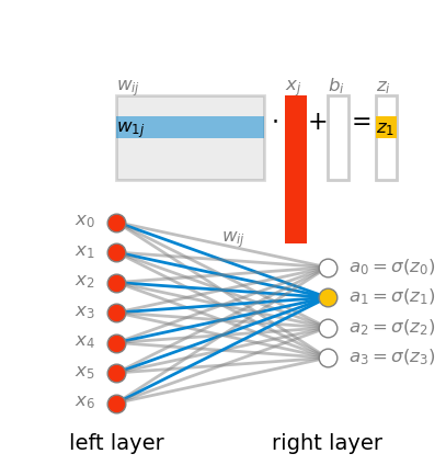
Pay attention the the order of indices in the weight matrix w. The first index corresponds to the layer on the right, and the second index corresponds to the layer on the left. It would be more intuitive if it were the other way around: first input then output. Sadly, If we want to multiply the weight matrix w by the input vector x, this is what we have to do. I’m saying this now because in the next chapter we’ll talk about backpropagation, and there I’ll discuss how to make it work with all the inputs in a mini-batch at once, by taking advantage of matrix multiplication. We’ll see then that the more natural order can, and will be used.
59.9 the code
This is exactly the same code as in the book. I only made minor updates to make it compatible with python3. In the next chapter I’ll go wild and take charge of this code, making it more modern and efficient.
Show the code
class Network(object):

    def __init__(self, sizes):
        """The list ``sizes`` contains the number of neurons in the
        respective layers of the network.  For example, if the list
        was [2, 3, 1] then it would be a three-layer network, with the
        first layer containing 2 neurons, the second layer 3 neurons,
        and the third layer 1 neuron.  The biases and weights for the
        network are initialized randomly, using a Gaussian
        distribution with mean 0, and variance 1.  Note that the first
        layer is assumed to be an input layer, and by convention we
        won't set any biases for those neurons, since biases are only
        ever used in computing the outputs from later layers."""
        self.num_layers = len(sizes)
        self.sizes = sizes
        self.biases = [np.random.randn(y, 1) for y in sizes[1:]]
        self.weights = [np.random.randn(y, x)
                        for x, y in zip(sizes[:-1], sizes[1:])]

    def feedforward(self, a):
        """Return the output of the network if ``a`` is input."""
        for b, w in zip(self.biases, self.weights):
            a = sigmoid(np.dot(w, a)+b)
        return a

    def SGD(self, training_data, epochs, mini_batch_size, eta,
            test_data=None):
        """Train the neural network using mini-batch stochastic
        gradient descent.  The ``training_data`` is a list of tuples
        ``(x, y)`` representing the training inputs and the desired
        outputs.  The other non-optional parameters are
        self-explanatory.  If ``test_data`` is provided then the
        network will be evaluated against the test data after each
        epoch, and partial progress printed out.  This is useful for
        tracking progress, but slows things down substantially."""
        if test_data: n_test = len(test_data)
        n = len(training_data)
        for j in range(epochs):
            random.shuffle(training_data)
            mini_batches = [
                training_data[k:k+mini_batch_size]
                for k in range(0, n, mini_batch_size)]
            for mini_batch in mini_batches:
                self.update_mini_batch(mini_batch, eta)
            if test_data:
                print("Epoch {0}: {1} / {2}".format(
                    j, self.evaluate(test_data), n_test))
            else:
                print("Epoch {0} complete".format(j))

    def update_mini_batch(self, mini_batch, eta):
        """Update the network's weights and biases by applying
        gradient descent using backpropagation to a single mini batch.
        The ``mini_batch`` is a list of tuples ``(x, y)``, and ``eta``
        is the learning rate."""
        nabla_b = [np.zeros(b.shape) for b in self.biases]
        nabla_w = [np.zeros(w.shape) for w in self.weights]
        for x, y in mini_batch:
            delta_nabla_b, delta_nabla_w = self.backprop(x, y)
            nabla_b = [nb+dnb for nb, dnb in zip(nabla_b, delta_nabla_b)]
            nabla_w = [nw+dnw for nw, dnw in zip(nabla_w, delta_nabla_w)]
        self.weights = [w-(eta/len(mini_batch))*nw
                        for w, nw in zip(self.weights, nabla_w)]
        self.biases = [b-(eta/len(mini_batch))*nb
                       for b, nb in zip(self.biases, nabla_b)]

    def backprop(self, x, y):
        """Return a tuple ``(nabla_b, nabla_w)`` representing the
        gradient for the cost function C_x.  ``nabla_b`` and
        ``nabla_w`` are layer-by-layer lists of numpy arrays, similar
        to ``self.biases`` and ``self.weights``."""
        nabla_b = [np.zeros(b.shape) for b in self.biases]
        nabla_w = [np.zeros(w.shape) for w in self.weights]
        # feedforward
        activation = x
        activations = [x] # list to store all the activations, layer by layer
        zs = [] # list to store all the z vectors, layer by layer
        for b, w in zip(self.biases, self.weights):
            z = np.dot(w, activation)+b
            zs.append(z)
            activation = sigmoid(z)
            activations.append(activation)
        # backward pass
        delta = self.cost_derivative(activations[-1], y) * \
            sigmoid_prime(zs[-1])
        nabla_b[-1] = delta
        nabla_w[-1] = np.dot(delta, activations[-2].transpose())
        # Note that the variable l in the loop below is used a little
        # differently to the notation in Chapter 2 of the book.  Here,
        # l = 1 means the last layer of neurons, l = 2 is the
        # second-last layer, and so on.  It's a renumbering of the
        # scheme in the book, used here to take advantage of the fact
        # that Python can use negative indices in lists.
        for l in range(2, self.num_layers):
            z = zs[-l]
            sp = sigmoid_prime(z)
            delta = np.dot(self.weights[-l+1].transpose(), delta) * sp
            nabla_b[-l] = delta
            nabla_w[-l] = np.dot(delta, activations[-l-1].transpose())
        return (nabla_b, nabla_w)

    def evaluate(self, test_data):
        """Return the number of test inputs for which the neural
        network outputs the correct result. Note that the neural
        network's output is assumed to be the index of whichever
        neuron in the final layer has the highest activation."""
        test_results = [(np.argmax(self.feedforward(x)), y)
                        for (x, y) in test_data]
        return sum(int(x == y) for (x, y) in test_results)

    def cost_derivative(self, output_activations, y):
        """Return the vector of partial derivatives \partial C_x /
        \partial a for the output activations."""
        return (output_activations-y)

#### Miscellaneous functions
def sigmoid(z):
    """The sigmoid function."""
    return 1.0/(1.0+np.exp(-z))

def sigmoid_prime(z):
    """Derivative of the sigmoid function."""
    return sigmoid(z)*(1-sigmoid(z))
Show the code
epochs = 10
net = Network([784, 30, 10])
start = time.perf_counter()
net.SGD(training_data,
        epochs=epochs,
        mini_batch_size=10,
        eta=3.0,
        test_data=test_data)
end = time.perf_counter()
print(f"Runtime: {end - start:.2f} seconds")
print(f"Average runtime per epoch: {(end - start) / epochs:.2f} seconds")
Epoch 0: 9096 / 10000
Epoch 1: 9263 / 10000
Epoch 2: 9296 / 10000
Epoch 3: 9354 / 10000
Epoch 4: 9396 / 10000
Epoch 5: 9433 / 10000
Epoch 6: 9453 / 10000
Epoch 7: 9456 / 10000
Epoch 8: 9470 / 10000
Epoch 9: 9453 / 10000
Runtime: 125.26 seconds
Average runtime per epoch: 12.53 seconds59.10 exercise H
NN with two layers only
Try creating a network with just two layers - an input and an output layer, no hidden layer - with 784 and 10 neurons, respectively. Train the network using stochastic gradient descent. What classification accuracy can you achieve?
net = Network([784, 10])
net.SGD(training_data,
        epochs=10,
        mini_batch_size=10,
        eta=3.0,
        test_data=test_data)
Epoch 0: 7506 / 10000
Epoch 1: 7592 / 10000
Epoch 2: 8220 / 10000
Epoch 3: 8279 / 10000
Epoch 4: 8308 / 10000
Epoch 5: 8321 / 10000
Epoch 6: 8325 / 10000
Epoch 7: 8333 / 10000
Epoch 8: 8373 / 10000
Epoch 9: 8294 / 10000