17 Spatial distribution - lecture

17.1 The problem

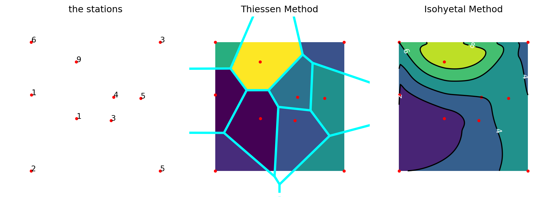
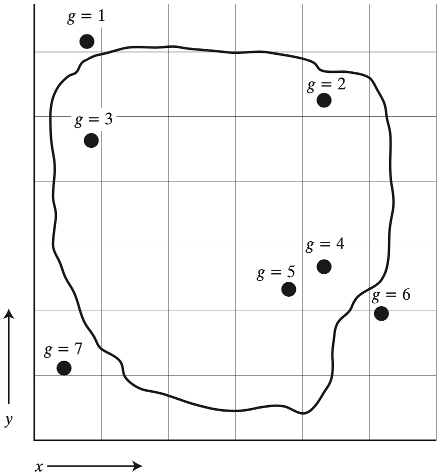
Let’s say we want to calculate the average rainfall on a watershed, and we have data available for 7 stations, as shown in the figure below [Dingman, figure 4.26]:

There are a number of methods for calculating the average precipitation.

17.2 Thiessen method [Voronoi diagram]

Brutsaert (2005), Figure 3.11

How to compute the areas:

Average areal precipitation is a weighted sum:

\langle P \rangle = \frac{\sum_i A_i P_i}{\sum_i A_i}

A nice way to understand the Thiessen method is depicted in this gif from Wikipedia.

17.3 Inverse distance method

Brutsaert (2005), Figure 3.12

The precipitation for square 17 is

P_{17} = \displaystyle\frac {\displaystyle\sum_\text{$i$ = all stations}\frac{P_i}{d_{i,17}^2}} {\displaystyle\sum_\text{$i$ = all stations}\frac{1}{d_{i,17}^2}}

The average precipitation for the whole watershed is the weighted average of all squares, where the weight is their area:

\langle P \rangle = \displaystyle\frac {\displaystyle\sum_\text{$j$ = all squares} A_j P_j} {\displaystyle\sum_\text{$j$ = all squares} A_j}

Brutsaert (2005), page 93:

Dean and Snyder (1977) found that the exponent (for the distance d^{-b}) b = 2 yielded the best results in the Piedmont region of the southeastern United States, whereas Simanton and Osborn (1980) concluded from measurements in Arizona that b can range between 1 and 3 without significantly affecting the results.

17.4 Isohyetal method

Brutsaert (2005), Figure 3.12

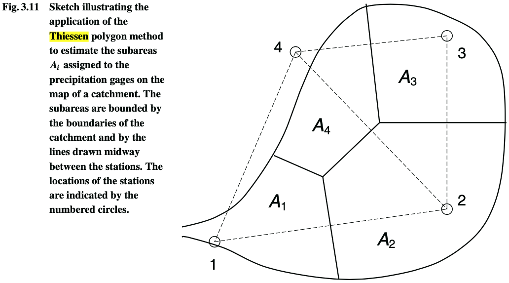
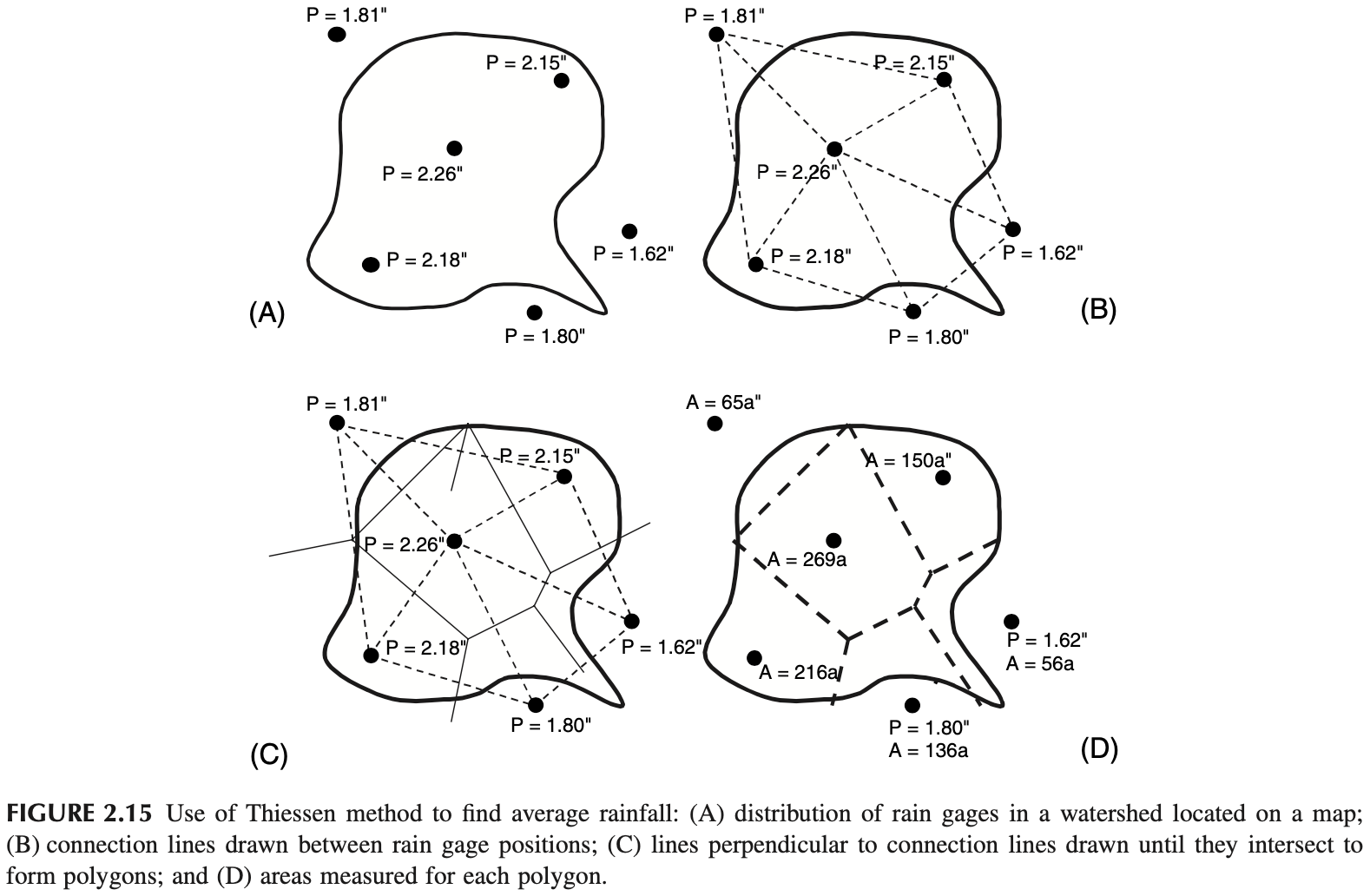
The same equation of the Thiessen method can be used:

\langle P \rangle = \frac{\sum_i A_i P_i}{\sum_i A_i}

17.5 How it is actually done

Most often, Geographic Information System (GIS) software is used to analyze spatial data. Two of the most used programs are ArcGIS (proprietary) and QGIS (free).

A good discussion of the different methods can be found on Manuel Gimond’s website, Intro to GIS and Spatial Analysis.

Attention!
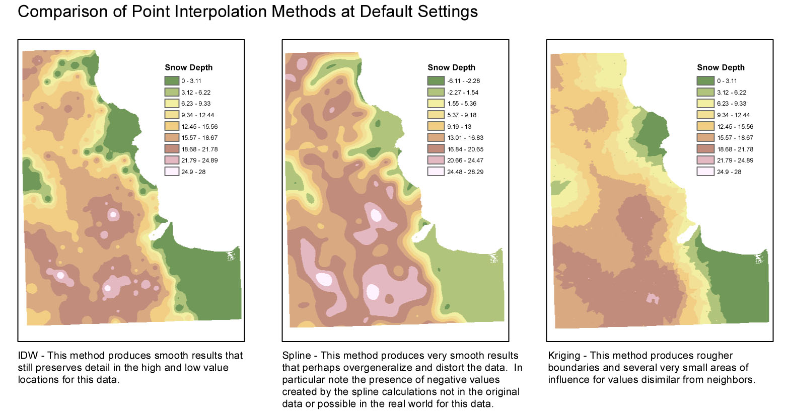
Don’t mix precision with accuracy. There are many ways of interpolating, just because a result seems detailed, it does not imply that it is accurate! See below three interpolation methods.

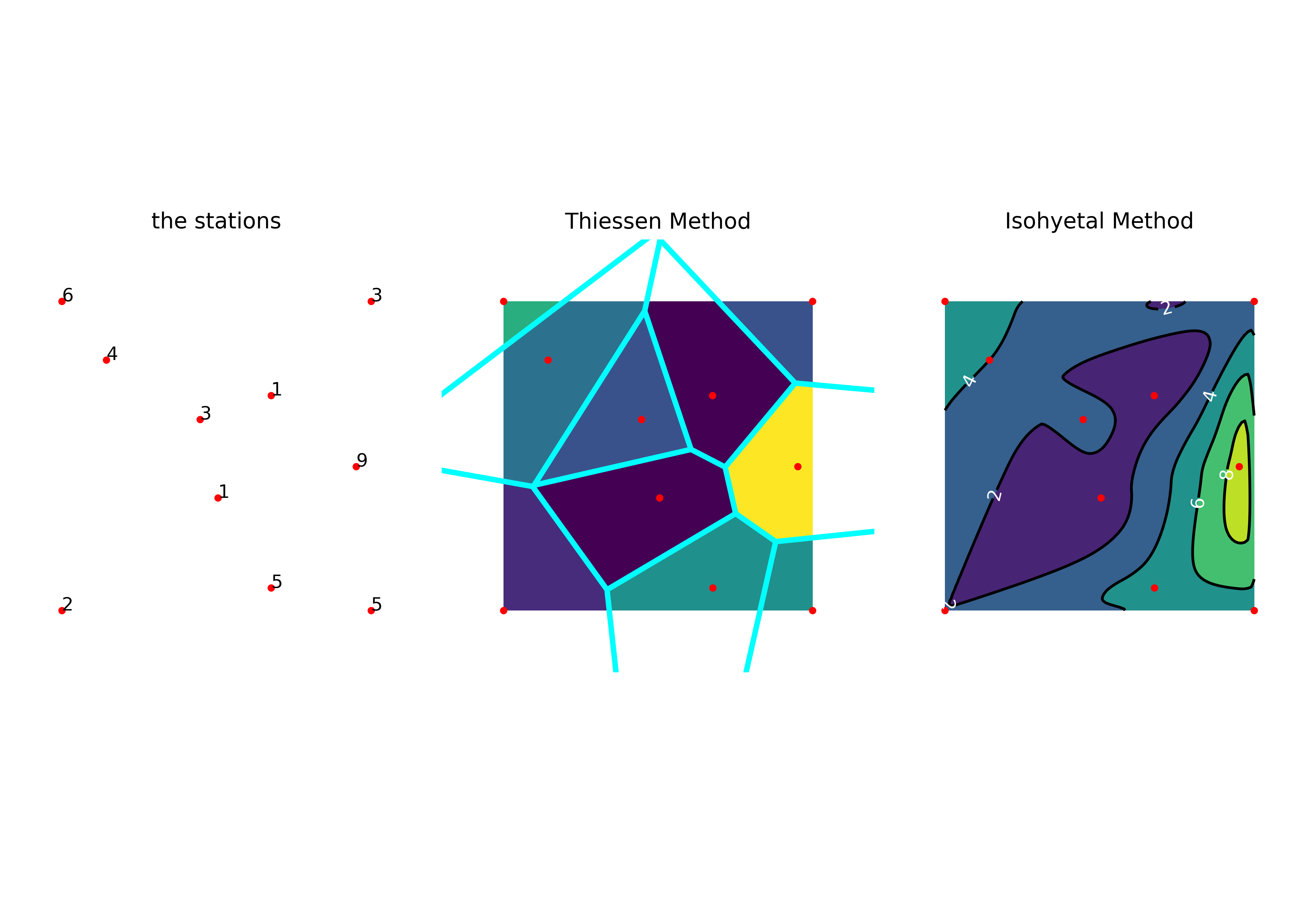
Below you can find a simple Python code that exemplifies some of the methods, producing the following figure:

Show the code

import matplotlib.pyplot as plt
import numpy as np
from scipy.interpolate import griddata
from scipy.spatial import Voronoi, voronoi_plot_2d, ConvexHull

fig, ax = plt.subplots(1, 3, figsize=(10,7))
fig.subplots_adjust(left=0.0, right=1.0, top=0.96, bottom=0.05,
                    hspace=0.02, wspace=0.02)

N = 6
PI = '3141592653589793'
points = np.random.rand(N, 2)
points = np.vstack([points,[0,0], [0,1], [1,0], [1,1]])
values = np.array([int(x) for x in list(PI)])[:(N+4)]
# values = np.array([3, 1, 4, 1, 5, 9, 2, 6, 5, 3])

grid_x, grid_y = np.mgrid[0:1:100j, 0:1:200j]

grid_z_nearest = griddata(points, values, (grid_x, grid_y), method='nearest')
grid_z_cubic = griddata(points, values, (grid_x, grid_y), method='cubic')

ax[0].plot(points[:,0], points[:,1], 'o', ms=3, markerfacecolor="red", markeredgecolor="red")
ax[0].set_aspect('equal', 'box')
ax[0].set(xlim=[0,1], ylim=[0,1])
ax[0].set_title("the stations")
for i, v in enumerate(values):
    ax[0].text(points[i,0], points[i,1], str(v))

ax[1].imshow(grid_z_nearest.T, extent=(0,1,0,1), origin='lower')
ax[1].plot(points[:,0], points[:,1], 'o', ms=3, markerfacecolor="red", markeredgecolor="red")
vor = Voronoi(points)
voronoi_plot_2d(vor, show_vertices=False, line_colors='cyan',
                line_width=3, line_alpha=1, point_size=0, ax=ax[1])
ax[1].set_title("Thiessen Method")

ax[2].plot(points[:,0], points[:,1], 'o', ms=3, markerfacecolor="red", markeredgecolor="red")
nlines = int((values.max()-values.min()+1)/2)
ax[2].contourf(grid_x, grid_y, grid_z_cubic, nlines)
cont = ax[2].contour(grid_x, grid_y, grid_z_cubic, nlines, colors="black")
ax[2].clabel(cont, inline=1, colors='white', fmt='%.0f')
ax[2].set_title("Isohyetal Method")

for i, a in enumerate(ax):
    a.set(xlim=[-0.2,1.2], ylim=[-0.2,1.2])
    a.axis('off')
    a.set_aspect('equal', 'box')

fig.savefig("spatial-distribution.png", dpi=500)