Find station codes in this map. On the left, click on the little wrench next to “Global Summary of the Month”, then click on “identify” on the panel that just opened, and click on a station (purple circle). You will see the station’s name, it’s ID, and the period of record. For example, for Ben-Gurion’s Airport in Israel:
BEN GURION, IS
STATION ID: ISM00040180
Period of Record: 1951-01-01 to 2020-03-01
You can download daily or monthly data for each station. Use the function below to download this data to your computer. station_name can be whatever you want, station_code is the station ID.
If everything fails and you need easy access to the files we’ll be using today, click here: Eilat daily.
Show the code
def download_data(station_name, station_code): url_daily ='https://www.ncei.noaa.gov/data/global-historical-climatology-network-daily/access/' url_monthly ='https://www.ncei.noaa.gov/data/gsom/access/'# download daily data - uncomment the following 2 lines to make this work urllib.request.urlretrieve(url_daily + station_code +'.csv', station_name +'_daily.csv')# download monthly data urllib.request.urlretrieve(url_monthly + station_code +'.csv', station_name +'_monthly.csv')
Download daily rainfall data for Eilat, Israel. ID: IS000009972
Show the code
download_data('Eilat', 'IS000009972')
Then load the data into a dataframe. IMPORTANT!! daily precipitation data is in tenths of mm, divide by 10 to get it in mm.
How do we know that? It’s in the documentation!
Show the code
df = pd.read_csv('Eilat_daily.csv', sep=",")# make 'DATE' the dataframe indexdf['DATE'] = pd.to_datetime(df['DATE'])df = df.set_index('DATE')# IMPORTANT!! daily precipitation data is in tenths of mm, divide by 10 to get it in mm.df['PRCP'] = df['PRCP'] /10df
STATION
LATITUDE
LONGITUDE
ELEVATION
NAME
PRCP
PRCP_ATTRIBUTES
TMAX
TMAX_ATTRIBUTES
TMIN
TMIN_ATTRIBUTES
TAVG
TAVG_ATTRIBUTES
DATE
1949-11-30
IS000009972
29.55
34.95
12.0
ELAT, IS
0.0
,,E
NaN
NaN
NaN
NaN
NaN
NaN
1949-12-01
IS000009972
29.55
34.95
12.0
ELAT, IS
0.0
,,E
NaN
NaN
NaN
NaN
NaN
NaN
1949-12-02
IS000009972
29.55
34.95
12.0
ELAT, IS
0.0
,,E
NaN
NaN
NaN
NaN
NaN
NaN
1949-12-03
IS000009972
29.55
34.95
12.0
ELAT, IS
0.0
,,E
NaN
NaN
NaN
NaN
NaN
NaN
1949-12-04
IS000009972
29.55
34.95
12.0
ELAT, IS
0.0
,,E
NaN
NaN
NaN
NaN
NaN
NaN
...
...
...
...
...
...
...
...
...
...
...
...
...
...
2024-01-16
IS000009972
29.55
34.95
12.0
ELAT, IS
NaN
NaN
231.0
,,S
108.0
,,S
170.0
H,,S
2024-01-17
IS000009972
29.55
34.95
12.0
ELAT, IS
NaN
NaN
211.0
,,S
117.0
,,S
164.0
H,,S
2024-01-18
IS000009972
29.55
34.95
12.0
ELAT, IS
NaN
NaN
240.0
,,S
111.0
,,S
174.0
H,,S
2024-01-19
IS000009972
29.55
34.95
12.0
ELAT, IS
NaN
NaN
244.0
,,S
135.0
,,S
182.0
H,,S
2024-01-20
IS000009972
29.55
34.95
12.0
ELAT, IS
NaN
NaN
NaN
NaN
118.0
,,S
147.0
H,,S
27072 rows × 13 columns
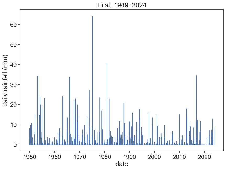
Plot precipitation data (‘PRCP’ column) and see if everything is all right.
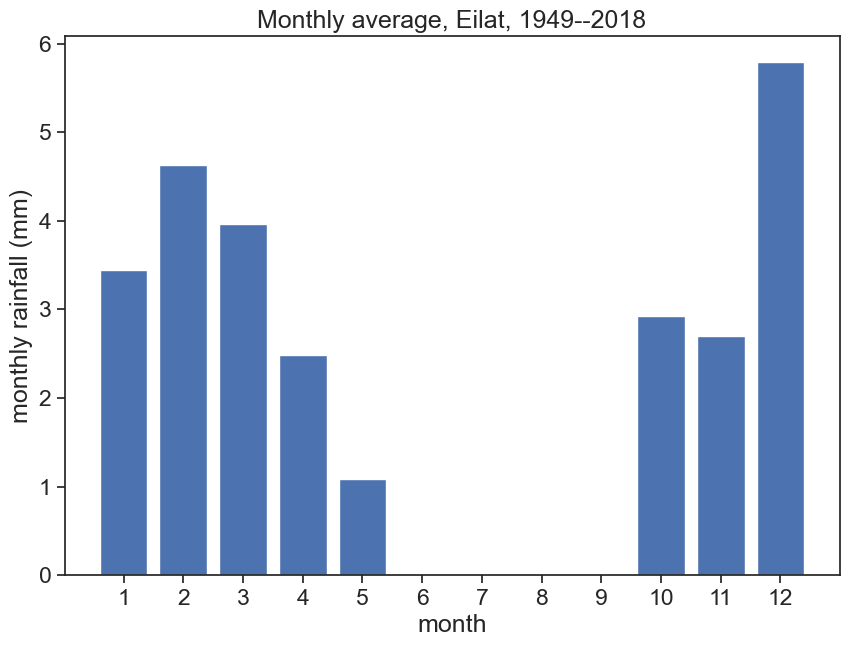
The rainfall data for Eilat is VERY seasonal, it’s easy to see that there is no rainfall at all during the summer. We can assume a hydrological year starting on 1 August. If you’re not sure, you can plot the monthly means (see last week’s lecture) and find what date makes sense best.
/var/folders/c3/7hp0d36n6vv8jc9hm2440__00000gn/T/ipykernel_71663/1784230487.py:1: FutureWarning: 'M' is deprecated and will be removed in a future version, please use 'ME' instead.
  df_month = df['PRCP'].resample('M').sum().to_frame()
/var/folders/c3/7hp0d36n6vv8jc9hm2440__00000gn/T/ipykernel_71663/299619059.py:1: FutureWarning: 'A-JUL' is deprecated and will be removed in a future version, please use 'YE-JUL' instead.
  max_annual = (df['PRCP'].resample('A-JUL')
PRCP
DATE
1951-07-31
10.8
1952-07-31
15.0
1953-07-31
34.4
1954-07-31
24.3
1955-07-31
19.0
...
...
2015-07-31
2.4
2016-07-31
8.5
2017-07-31
34.5
2018-07-31
11.7
2019-07-31
0.0
69 rows × 1 columns
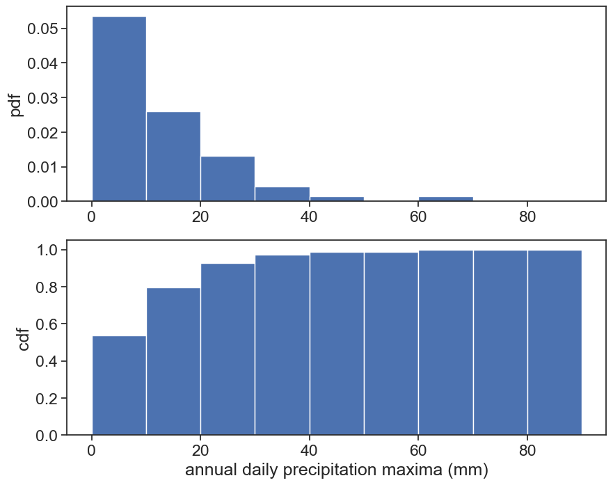
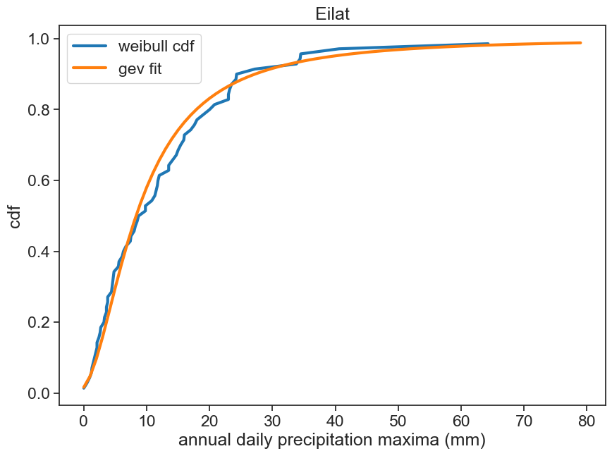
Make two graphs: a) the histogram for the annual maximum (pdf) b) the cumulative probability (cdf)
# sort the annual daily precipitation maxima, from lowest to highestmax_annual['max_sorted'] = np.sort(max_annual['PRCP'])# let's give it a name, hh = max_annual['max_sorted'].values# make an array "order" of size N=len(h), from 1 to NN =len(h)rank = np.arange(N) +1# make a new array, "rank"cdf_weibull = rank / (N+1)
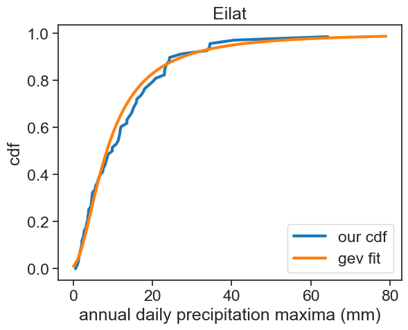
Plot it next to the cdf that pandas’ hist makes for you. What do you see?
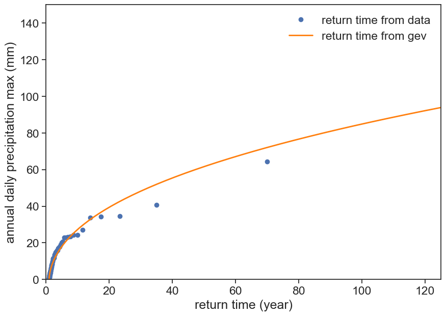
We are almost there! Remember that the return time are given by:
T_r(x) = \frac{1}{1-F(x)},
where F is the cdf.
Survival = 1-F
The package that we are using, scipy.stats.genextreme has a method called isf, or inverse survival function, which is exactly what we want! In order to use it, you have to feed it a “quantile” q or probability. Suppose you want to know how strong is a 1 in a 100 year event, then your return period is 100 (years), and the probability is simply its inverse, 1/100.
cdf as we are use to
fig, ax = plt.subplots(figsize=(10,7))T =1/ (1-cdf_weibull)ax.plot(T, h, 'o', label="return time from data")rain = np.arange(0,150)cdf_rain = genextreme(c=params[0], loc=params[1], scale=params[2]).cdf(rain)ax.plot(1/(1-cdf_rain), rain, color='tab:orange', lw=2, label="return time from gev")ax.legend(loc="upper right", frameon=False)ax.set(xlabel="return time (year)", ylabel=f"annual daily precipitation max (mm)", xlim=[0, 125], ylim=[0, 150]);
In the code below, we use 1/T as the argument for isf. Why?
We know that
T = \frac{1}{1-\text{CDF}} = \frac{1}{\text{SF}}
If we take the reciprocal of the equation above, SF will become the inverse SF, or ISF:
You might want to do the opposite: given a list of critical daily max levels, what are the return periods for them? In this case you can use the sf method, “survival function”.
Not always the fit operation succeeds. Sometimes, the fitted parameters yield curves that do not seem to describe well the pdf or the cdf we are studying. What to do?
ALWAYS check your parameters. Plot the fitted curve against the experimental data and see with your eyes if it makes sense.
If it doesn’t make sense, you have to run fit again, with some changes. A common problem is that the algorithm chose initial values for the parameters that do not converge to the optimal parameters we are looking for. In this case, one needs to help fit by giving it initial guesses for the parameters, like this: