4 Exercises
Import relevant packages
4.1 intra-annual variability
Go to NOAA’s National Centers for Environmental Information (NCEI)
Climate Data Online: Dataset Discovery
Find station codes in this map. On the left, click on the little wrench (🔧) next to “Global Summary of the Month”, then click on “identify” on the panel that just opened, and click on a station (purple circle). You will see the station’s name, it’s ID, and the period of record. For example, for Ben-Gurion’s Airport in Israel:
BEN GURION, IS
STATION ID: ISM00040180
Period of Record: 1951-01-01 to 2020-03-01
You can download daily or monthly data for each station. Use the function below to download this data to your computer.
If everything fails and you need easy access to the files we’ll be using today, click here:
Ben Gurion, Beer Sheva.
def download_data(station_name, station_code):
    url_daily = 'https://www.ncei.noaa.gov/data/global-historical-climatology-network-daily/access/'
    url_monthly = 'https://www.ncei.noaa.gov/data/gsom/access/'
    # download daily data - uncomment the next 2 lines to make this work
    # urllib.request.urlretrieve(url_daily + station_code + '.csv',
    #                            station_name + '_daily.csv')
    # download monthly data
    urllib.request.urlretrieve(url_monthly + station_code + '.csv',
station_name + '_monthly.csv')Now, choose any station with a period of record longer than 30 years, and download its data:
Load the data into a datafram, and before you continue with the analysis, plot the rainfall data, to see how it looks like.
download_data('BEN_GURION', 'ISM00040180')
df = pd.read_csv('BEN_GURION_monthly.csv', sep=",")
# make 'DATE' the dataframe index
df['DATE'] = pd.to_datetime(df['DATE'])
df = df.set_index('DATE')
plt.plot(df['PRCP']);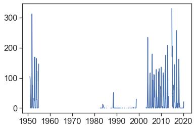
It doesn’t look great for Ben-Gurion airport, lots of missing data! You might need to choose another station…
ALWAYS look at your data to see if it looks good.
NEVER mindlessly run code on data you don’t know to be good.
Download data for Beer Sheva, ID IS000051690.
download_data('BEER_SHEVA', 'IS000051690')
df = pd.read_csv('BEER_SHEVA_monthly.csv', sep=",")
# make 'DATE' the dataframe index
df['DATE'] = pd.to_datetime(df['DATE'])
df = df.set_index('DATE')
plt.plot(df['PRCP']);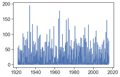
That’s much better! We need to aggregate all data from each month, so we can calculate monthly averages. How to do that?
group_by_month = df['PRCP'].groupby(df.index.month)
df_beersheva = (group_by_month
                  .mean()
                  .to_frame()
               )
df_beersheva = df_beersheva.reset_index()
df_beersheva.columns = ['month number', 'monthly rainfall (mm)']
df_beersheva| month number | monthly rainfall (mm) | |
|---|---|---|
| 0 | 1 | 48.743158 |
| 1 | 2 | 37.347368 |
| 2 | 3 | 26.551579 |
| 3 | 4 | 9.038947 |
| 4 | 5 | 2.735789 |
| 5 | 6 | 0.013830 |
| 6 | 7 | 0.000000 |
| 7 | 8 | 0.002128 |
| 8 | 9 | 0.271277 |
| 9 | 10 | 6.669474 |
| 10 | 11 | 21.850526 |
| 11 | 12 | 41.786316 |
groupby is a very powerful tool, but it takes some time to get used to it. We usually make operations on the groupby object like this:
If you try to see the object group_by_month you won’t see anything. This object waits for further instructions to be useful. Another way of understanding what’s going on with this operation is to see with our eyes one of the groups:
If you want to calculate the same averages using a loop instead of groupby, then you can do the following:
# choose only the precipitation column
df_month = df['PRCP']
# calculate monthly mean
monthly_mean = np.array([])  # empty array
month_numbers = np.arange(1,13)

for m in month_numbers:      # cycle over months (1, 2, 3, etc)
    this_month_all_indices = (df_month.index.month == m)       # indices in df_month belonging to month m
    this_month_mean = df_month[this_month_all_indices].mean()  # this is the monthly mean
    monthly_mean = np.append(monthly_mean, this_month_mean)    # append

df_beersheva = pd.DataFrame({'monthly rainfall (mm)':monthly_mean,
                             'month number':month_numbers
                            })
df_beersheva| monthly rainfall (mm) | month number | |
|---|---|---|
| 0 | 48.743158 | 1 |
| 1 | 37.347368 | 2 |
| 2 | 26.551579 | 3 |
| 3 | 9.038947 | 4 |
| 4 | 2.735789 | 5 |
| 5 | 0.013830 | 6 |
| 6 | 0.000000 | 7 |
| 7 | 0.002128 | 8 |
| 8 | 0.271277 | 9 |
| 9 | 6.669474 | 10 |
| 10 | 21.850526 | 11 |
| 11 | 41.786316 | 12 |
Plot the data and see if it makes sense. Try to get a figure like this one.
fig, ax = plt.subplots(figsize=(10,7))
ax.bar(df_beersheva['month number'], df_beersheva['monthly rainfall (mm)'])
ax.set(xlabel="months",
       ylabel="monthly average (mm)",
       title="Beer Sheva",
       xticks=df_beersheva['month number'],
       xticklabels=df_beersheva['month number']);
# plt.savefig("beersheva_monthly_average.png")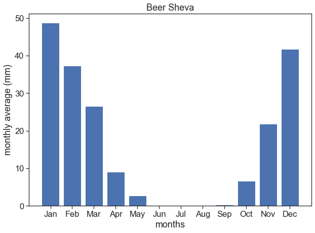
Let’s calculate now the Walsh and Lawler Seasonality Index: leddris (2010), Walsh and Lawler (1981).
Write a function that receives a dataframe like the one we have just created, and returns the seasonality index.
R= mean annual precipitation
m_i= precipitation mean for month i
SI = \displaystyle \frac{1}{R} \sum_{n=1}^{n=12} \left| m_i - \frac{R}{12} \right|
| SI | Precipitation Regime |
|---|---|
| <0.19 | Precipitation spread throughout the year |
| 0.20-0.39 | Precipitation spread throughout the year, but with a definite wetter season |
| 0.40-0.59 | Rather seasonal with a short dry season |
| 0.60-0.79 | Seasonal |
| 0.80-0.99 | Marked seasonal with a long dry season |
| 1.00-1.19 | Most precipitation in < 3 months |