import matplotlib.pyplot as pltimport matplotlibimport numpy as npimport pandas as pdfrom pandas.plotting import register_matplotlib_convertersregister_matplotlib_converters() # datetime converter for a matplotlibfrom calendar import month_abbrimport seaborn as snssns.set_theme(style="ticks", font_scale=1.5)import urllib.requestimport matplotlib.dates as mdates
---------------------------------------------------------------------------ModuleNotFoundError Traceback (most recent call last)
Cell In[1], line 9 7 register_matplotlib_converters() # datetime converter for a matplotlib 8fromcalendarimport month_abbr
----> 9importseabornassns 10 sns.set_theme(style="ticks", font_scale=1.5)
11importurllib.requestModuleNotFoundError: No module named 'seaborn'
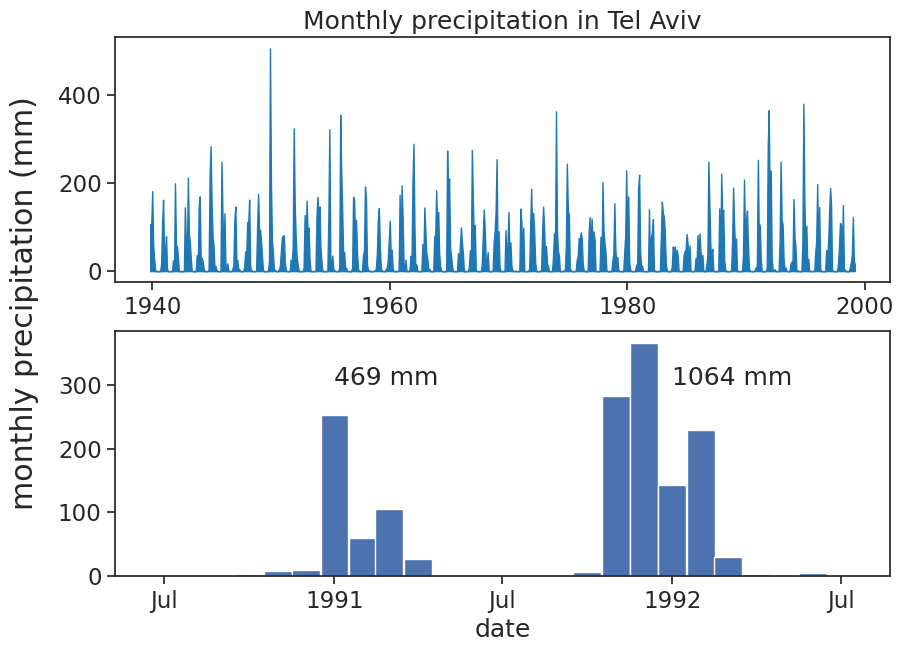
fig, (ax1, ax2) = plt.subplots(2, 1, figsize=(10,7))# plot precipitationax1.fill_between(df.index, df['PRCP'], 0, color='tab:blue')df_1990_1992 = df.loc['1990-07-01':'1992-07-01']ax2.bar(df_1990_1992.index, df_1990_1992['PRCP'], width=30)# adjust labels, ticks, title, etcax1.set_title("Monthly precipitation in Tel Aviv")# ax2.tick_params(axis='x', rotation=45)ax2.set_xlabel("date")concise(ax1)concise(ax2)# common y label between the two panels:fig.supylabel('monthly precipitation (mm)')# write yearly rainfallrain_1990_1991 = df.loc['1990-07-01':'1991-07-01','PRCP'].sum()rain_1991_1992 = df.loc['1991-07-01':'1992-07-01','PRCP'].sum()ax2.text('1991-01-01', 300, "{:.0f} mm".format(rain_1990_1991))ax2.text('1992-01-01', 300, "{:.0f} mm".format(rain_1991_1992))pass# save figure# plt.savefig("monthly_tel_aviv_1940-1999.png")
Let’s aggregate (resample) precipitation according to the hydrological year.
resample by hydrological year
# read more about resampling options# https://pandas.pydata.org/pandas-docs/version/0.12.0/timeseries.html#offset-aliases# also, annual resampling can be anchored to the end of specific months:# https://pandas.pydata.org/pandas-docs/version/0.12.0/timeseries.html#anchored-offsetsdf_year = df['PRCP'].resample('YE-SEP').sum().to_frame() # yearly frequency, anchored end of Septemberdf_year.columns = ['rain (mm)'] # rename 'PRCP' column to 'rain (mm)'# the last year is the sum of only on month (November), let's take it outdf_year = df_year.iloc[:-1] # exclude last row
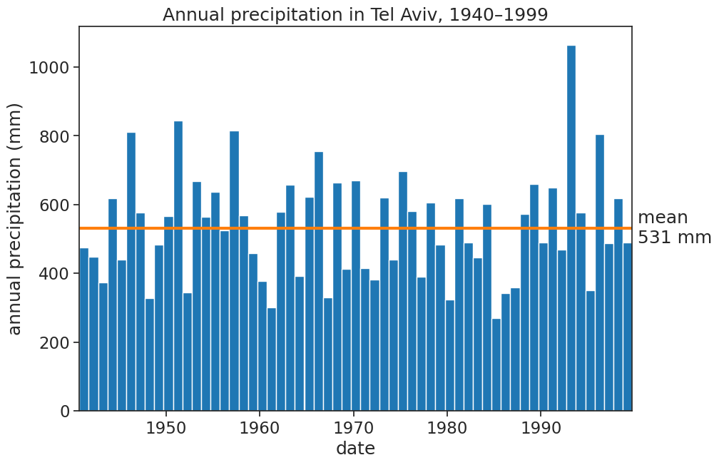
plot mean
fig, ax = plt.subplots(figsize=(10,7))# plot YEARLY precipitationax.bar(df_year.index, df_year['rain (mm)'], width=365, align='edge', color="tab:blue")# plot meanrain_mean = df_year['rain (mm)'].mean()ax.plot(df_year*0+ rain_mean, linewidth=3, color="tab:orange")# adjust labels, ticks, title, etcax.set(title="Annual precipitation in Tel Aviv, 1940–1999", xlabel="date", ylabel="annual precipitation (mm)", xlim=[df_year.index[0], df_year.index[-1]] )# write mean on the rightax.text(df_year.index[-1], rain_mean, " mean\n{:.0f} mm".format(rain_mean), horizontalalignment="left", verticalalignment="center");# save figure# plt.savefig("annual_tel_aviv_with_mean.png")
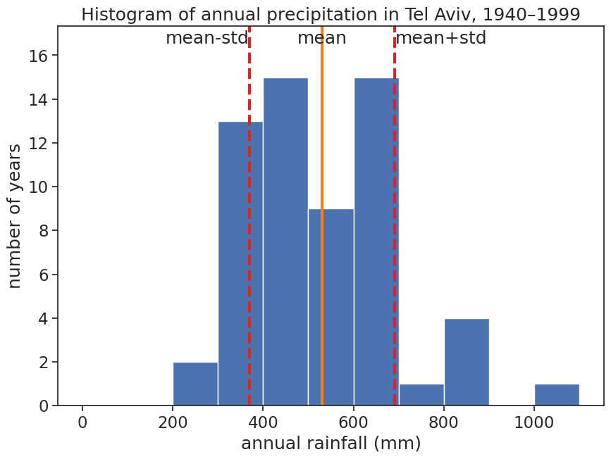
plot histogram
fig, ax = plt.subplots(figsize=(10,7))# calculate mean and standard deviationrain_mean = df_year['rain (mm)'].mean()rain_std = df_year['rain (mm)'].std()# plot histogramb = np.arange(0, 1101, 100) # bins from 0 to 55, width = 5ax.hist(df_year, bins=b)# plot vertical lines with mean, std, etcylim = np.array(ax.get_ylim())ylim[1] = ylim[1]*1.1ax.plot([rain_mean]*2, ylim, linewidth=3, color="tab:orange")ax.plot([rain_mean+rain_std]*2, ylim, linewidth=3, linestyle="--", color="tab:red")ax.plot([rain_mean-rain_std]*2, ylim, linewidth=3, linestyle="--", color="tab:red")ax.set_ylim(ylim)# write mean, std, etcax.text(rain_mean, ylim[1]*0.99, "mean", horizontalalignment="center", verticalalignment="top", )ax.text(rain_mean+rain_std, ylim[1]*0.99, "mean+std", horizontalalignment="left", verticalalignment="top", )ax.text(rain_mean-rain_std, ylim[1]*0.99, "mean-std", horizontalalignment="right", verticalalignment="top", )# adjust labels, ticks, title, limits, etcax.set(title="Histogram of annual precipitation in Tel Aviv, 1940–1999", xlabel="annual rainfall (mm)", ylabel="number of years" );# save figure# plt.savefig("histogram_tel_aviv_with_mean_and_std.png")
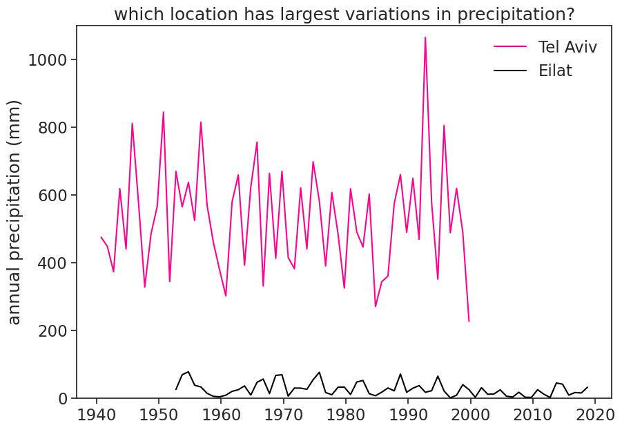
load and process data for Eilat
df_eilat = pd.read_csv("Eilat_monthly.csv", sep=",", parse_dates=['DATE'], index_col='DATE' )df_year_eilat = df_eilat['PRCP'].resample('YE-SEP').sum().to_frame() # yearly frequency, anchored end of Septemberdf_year_eilat.columns = ['rain (mm)'] # rename 'PRCP' column to 'rain (mm)'df_year_eilat = df_year_eilat.iloc[2:-5] # exclude first two and last two years
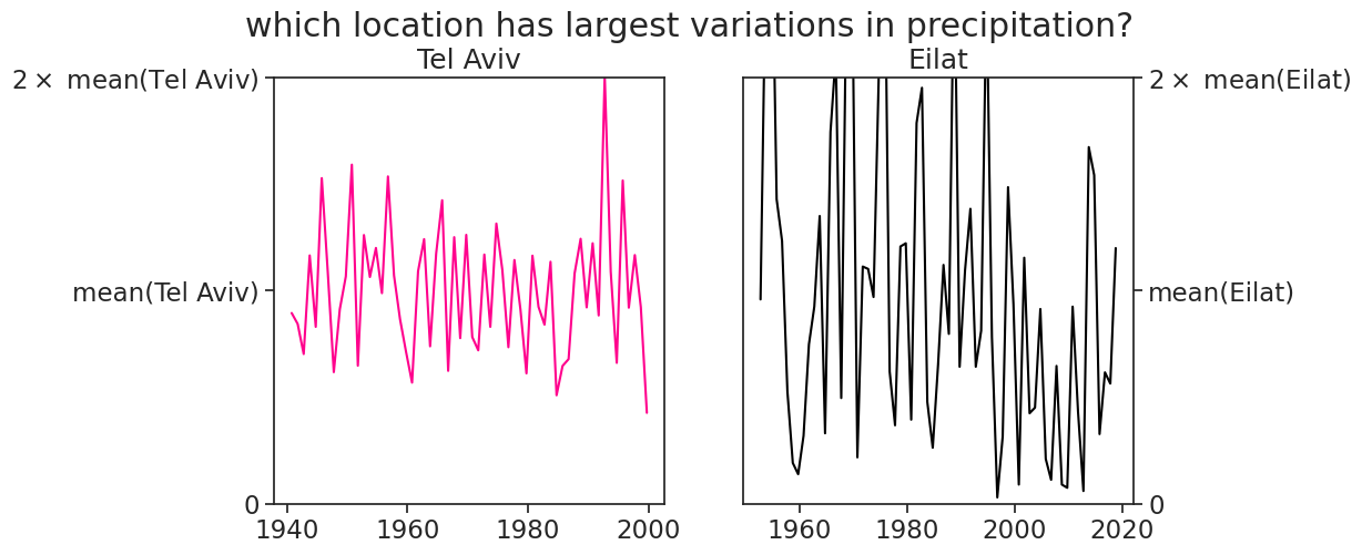
Text(0.5, 1.0, 'which location has largest variations in precipitation?')
5.1 coefficient of variation
\langle{P}\rangle= average precipitation \sigma= standard deviation
CV = \frac{\sigma}{\langle{P}\rangle}
The coefficient of variation (dimensionless) quantifies the variation (std) magnitude with respect to the mean. In the examples above, although Tel Aviv has a much higher standard deviation in annual precipitation, the spread of precipitation in Eilat is much larger, considered relative to its average.
Tel Aviv:   std = 161.19 mm     CV = 0.30
Eilat:      std = 20.49 mm      CV = 0.77
Another way to understand the CV: for gaussian (normal) distributions, 67% of the data lies 1 std from the mean. Assuming that the annual rainfall for Tel Aviv and Eilat roughly follows a gaussian distribution, we could say that:
Tel Aviv: about 67% of the annual precipitation is no more than 30% from the average.
Eilat: about 67% of the annual precipitation is no more than 77% from the average.
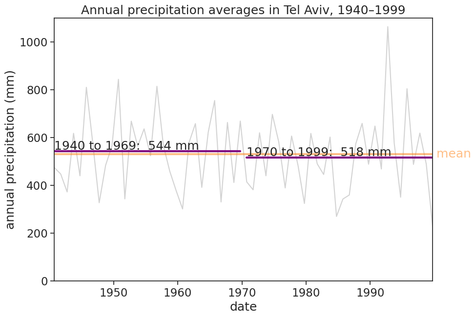
Normals serve two purposes: a reference period for monitoring current weather and climate, and a good description of the expected climate at a location over the seasons. They provide a basis for determining whether today’s weather is warmer or colder, wetter or drier. They also can be used to plan for conditions beyond the time span of reliable weather forecasts. A 30-year time period was chosen by the governing body of international meteorology in the 1930s, so the first normals were for 1901-1930, the longest period for which most countries had reliable climate records. International normals were called for in 1931-1960 and 1961-1990, but many countries updated normals more frequently, every 10 years, so as to keep them up to date. In 2015 this was made the WMO standard, so all countries will be creating normals for 1991-2020.
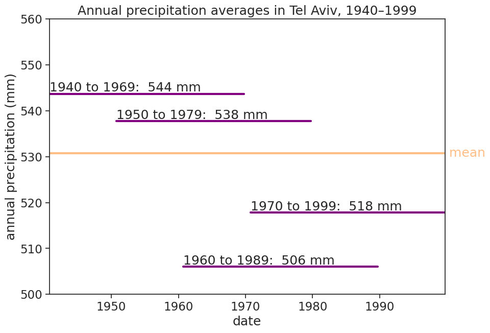
fig, ax = plt.subplots(figsize=(10,7))# windows of length 30 yearswindows = [[x,x+29] for x in [1940,1950,1960,1970]]for window in windows: start_date =f"{window[0]:d}-09-30" end_date =f"{window[1]:d}-09-30" window_mean = df_year['rain (mm)'][start_date:end_date].mean() ax.plot(df_year[start_date:end_date]*0+window_mean, color="purple", linewidth=3) ax.text(start_date, window_mean+0.5, f"{window[0]} to {window[1]}: {window_mean:.0f} mm",)# plot meanrain_mean = df_year['rain (mm)'].mean()ax.plot(df_year*0+ rain_mean, linewidth=3, color="tab:orange", alpha=0.5)ax.text(df_year.index[-1], rain_mean, " mean".format(rain_mean), horizontalalignment="left", verticalalignment="center", color="tab:orange", alpha=0.5)# adjust labels, ticks, title, limits, etcax.set(title="Annual precipitation averages in Tel Aviv, 1940–1999", xlabel="date", ylabel="annual precipitation (mm)", xlim=[df_year.index[0], df_year.index[-1]], ylim=[500, 560], );# save figure# plt.savefig("mean_tel_aviv_2_windows.png")
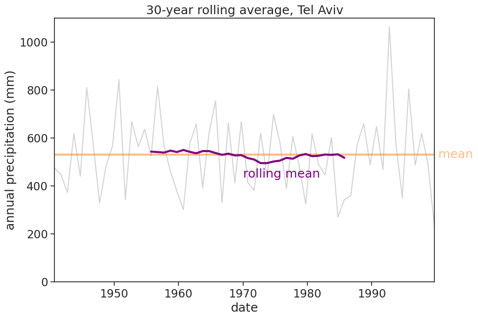
widget for rolling average
import altair as alt# Custom theme for readabilitydef readable(): return {"config" : {"title": {'fontSize': 16},"axis": {"labelFontSize": 16,"titleFontSize": 16, },"header": {"labelFontSize": 14,"titleFontSize": 14, },"legend": {"labelFontSize": 14,"titleFontSize": 14, },"mark": {'fontSize': 14,"tooltip": {"content": "encoding"}, # enable tooltips }, } }alt.themes.register('readable', readable)alt.themes.enable('readable')# Altair only recognizes column data; it ignores index values. You can plot the index data by first resetting the indexsource = df_year.reset_index()brush = alt.selection_interval(encodings=['x'])# T: temporal, a time or date value# Q: quantitative, a continuous real-valued quantity# https://altair-viz.github.io/user_guide/encoding.html#encoding-data-typesbars = alt.Chart().mark_bar().encode( x=alt.X('DATE:T', axis=alt.Axis(title='date')), y=alt.Y('rain (mm):Q', axis=alt.Axis(title='annual precipitation (mm) and average')), opacity=alt.condition(brush, alt.OpacityValue(1), alt.OpacityValue(0.2)),).add_params( brush).properties( title='Select year range and drag for rolling average of annual precipitation in Tel Aviv').properties( width=600, height=400)line = alt.Chart().mark_rule(color='orange').encode( y='mean(rain (mm)):Q', size=alt.SizeValue(3)).transform_filter( brush)alt.layer(bars, line, data=source)