6 Exercises
Import relevant packages
Plot monthly rainfall for your station.
Load the data into a dataframe, and before you continue with the analysis, plot the rainfall data, to see how it looks like.
df = pd.read_csv('BEER_SHEVA_monthly.csv', sep=",")
# make 'DATE' the dataframe index
df['DATE'] = pd.to_datetime(df['DATE'])
df = df.set_index('DATE')

fig, (ax1, ax2) = plt.subplots(2, 1, figsize=(10,7))
ax1.plot(df['PRCP'])
ax2.plot(df['PRCP']['2010-07-01':'2015-07-01'])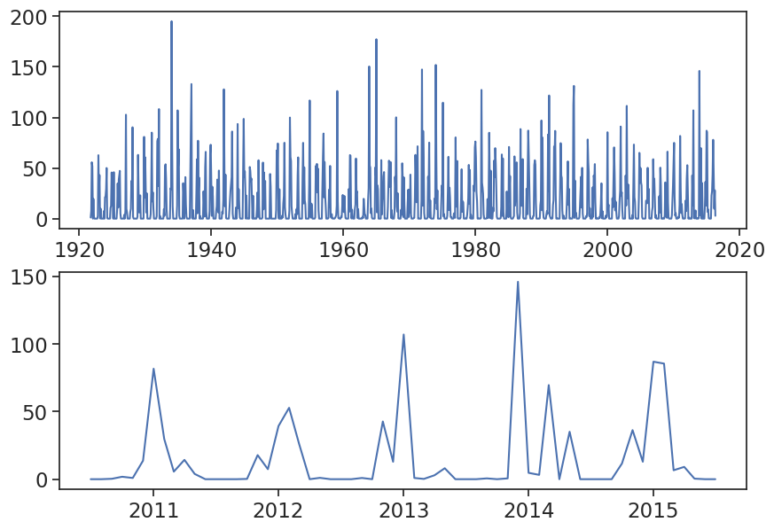
How to aggregate rainfall accoding to the hydrological year? We use the function resample.
read more about resampling options:
https://pandas.pydata.org/docs/user_guide/timeseries.html#offset-aliases
also, annual resampling can be anchored to the end of specific months: https://pandas.pydata.org/docs/user_guide/timeseries.html#anchored-offsets
# annual frequency, anchored 31 December
df_year_all = df['PRCP'].resample('YE').sum().to_frame()
# annual frequency, anchored 01 January
df_year_all = df['PRCP'].resample('YS').sum().to_frame()
# annual frequency, anchored end of September
df_year_all = df['PRCP'].resample('YE-SEP').sum().to_frame()
# rename 'PRCP' column to 'rain (mm)'
df_year_all.columns = ['rain (mm)']
df_year_all| rain (mm) | |
|---|---|
| DATE | |
| 1922-09-30 | 136.6 |
| 1923-09-30 | 144.5 |
| 1924-09-30 | 130.4 |
| 1925-09-30 | 165.3 |
| 1926-09-30 | 188.7 |
| ... | ... |
| 2012-09-30 | 145.7 |
| 2013-09-30 | 175.3 |
| 2014-09-30 | 259.2 |
| 2015-09-30 | 249.3 |
| 2016-09-30 | 257.6 |
95 rows × 1 columns
You might need to exclude the first or the last line, since their data might have less that 12 months. For example:
# exclude 1st row
df_year = df_year_all.iloc[1:]
# exclude last row
df_year = df_year_all.iloc[:-1]
# exclude both 1st and last rows
df_year = df_year_all.iloc[1:-1]
df_year| rain (mm) | |
|---|---|
| DATE | |
| 1923-09-30 | 144.5 |
| 1924-09-30 | 130.4 |
| 1925-09-30 | 165.3 |
| 1926-09-30 | 188.7 |
| 1927-09-30 | 130.2 |
| ... | ... |
| 2011-09-30 | 151.6 |
| 2012-09-30 | 145.7 |
| 2013-09-30 | 175.3 |
| 2014-09-30 | 259.2 |
| 2015-09-30 | 249.3 |
93 rows × 1 columns
Calculate the average annual rainfall. Plot annual rainfall for the whole range, together with the average. You should get something like this:
fig, ax = plt.subplots(figsize=(10,7))

# plot YEARLY precipitation
ax.bar(df_year.index, df_year['rain (mm)'],
       width=365, align='edge', color="tab:blue")

# plot mean
rain_mean = df_year['rain (mm)'].mean()
ax.plot(ax.get_xlim(), [rain_mean]*2, linewidth=3, color="tab:orange")
ax.set(xlabel="date",
       ylabel="yearly rainfall (mm)",
       title=f"Beer Sheva, mean = {rain_mean:.0f} mm");
# save figure
# plt.savefig("beersheva_yearly_rainfall_1923_2016.png")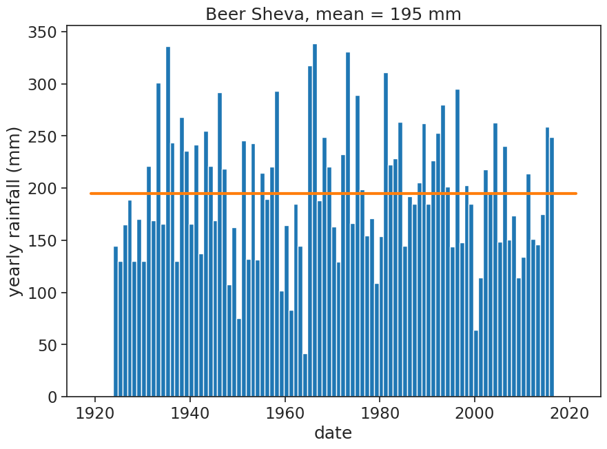
Plot a histogram of annual rainfall, with the mean and standard deviation. Calculate the coefficient of variation. Try to plot something like this:
fig, ax = plt.subplots(figsize=(10,7))

# calculate mean, standard deviation, CV
rain_mean = df_year['rain (mm)'].mean()
rain_std = df_year['rain (mm)'].std()
CV = rain_std/rain_mean
# plot histogram
b = np.arange(0, 401, 50)  # bins from 0 to 400, width = 50
ax.hist(df_year['rain (mm)'], bins=b)

# plot vertical lines with mean, std, etc
ylim = np.array(ax.get_ylim())
ylim[1] = ylim[1]*1.1
ax.plot([rain_mean]*2, ylim, linewidth=3, color="tab:orange")
ax.plot([rain_mean+rain_std]*2, ylim, linewidth=3, linestyle="--", color="tab:olive")
ax.plot([rain_mean-rain_std]*2, ylim, linewidth=3, linestyle="--", color="tab:olive")
ax.set(ylim=ylim,
       xlabel="annual rainfall (mm)",
       ylabel="number of years",
       title=f"Beer Sheva, 1922–2016. Mean={rain_mean:.0f} mm, STD={rain_std:.0f} mm")
ax.text(300, 25, f"CV = {CV:.2f}")
# plt.savefig("histogram_beersheva.png")
Text(300, 25, 'CV = 0.33')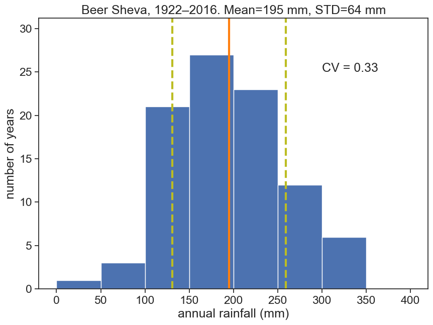
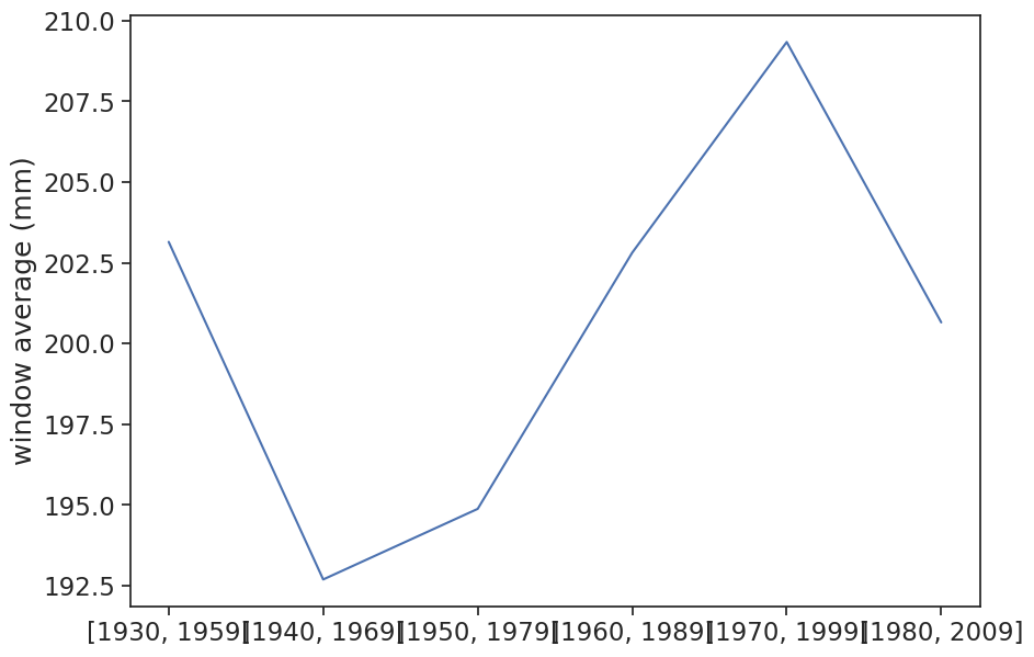
Calculate the mean annual rainfall for various 30-year intervals
####### the hard way #######
# fig, ax = plt.subplots(figsize=(10,7))

# mean_30_59 = df_year.loc['1930-09-30':'1959-09-01','rain (mm)'].mean()
# mean_40_69 = df_year.loc['1940-09-30':'1969-09-01','rain (mm)'].mean()
# mean_50_79 = df_year.loc['1950-09-30':'1979-09-01','rain (mm)'].mean()
# mean_60_89 = df_year.loc['1960-09-30':'1989-09-01','rain (mm)'].mean()
# mean_70_99 = df_year.loc['1970-09-30':'1999-09-01','rain (mm)'].mean()
# mean_80_09 = df_year.loc['1980-09-30':'2009-09-01','rain (mm)'].mean()

# ax.plot([mean_30_59,
#          mean_40_69,
#          mean_50_79,
#          mean_60_89,
#          mean_70_99,
#          mean_80_09])


####### the easy way #######

fig, ax = plt.subplots(figsize=(10,7))

# use list comprehension
windows = [[x, x+29] for x in [1930,1940,1950,1960,1970,1980]]
mean = [df_year.loc[f'{w[0]:d}-09-30':f'{w[1]:d}-09-01','rain (mm)'].mean() for w in windows]
ax.plot(mean)
ax.set(xticks=np.arange(len(mean)),
       xticklabels=[str(w) for w in windows],
       ylabel="window average (mm)"
      );