3 Intra-annual variability of precipitation
load data and process it
df_telaviv = pd.read_csv("TEL_AVIV_READING_monthly.csv",
                         sep=",",
                         parse_dates=['DATE'],
                         index_col='DATE'
                        )
df_london = pd.read_csv("LONDON_HEATHROW_monthly.csv",
                        sep=",",
                        parse_dates=['DATE'],
                        index_col='DATE'
                       )
monthly_london = (df_london['PRCP']
                   .groupby(df_london.index.month)
                   .mean()
                   .to_frame()
                  )
monthly_telaviv = (df_telaviv['PRCP']
                    .groupby(df_telaviv.index.month)
                    .mean()
                    .to_frame()
                  )
plot rainfall distribution
fig, ax = plt.subplots(figsize=(10,7))

# bar plots
ax.bar(monthly_london.index, monthly_london['PRCP'],
        alpha=0.5, color="blue", label=f"London ({monthly_london.values.sum():.0f} mm per year)")
ax.bar(monthly_telaviv.index, monthly_telaviv['PRCP'],
        alpha=0.5, color="red", width=0.5, label=f"Tel Aviv ({monthly_telaviv.values.sum():.0f} mm per year)")

# axes labels and figure title
ax.set(xlabel='month',
       ylabel='monthly rainfall average (mm)',
       title='seasonality of two cities with similar yearly rainfall',
       xticks=monthly_telaviv.index
      )
ax.legend(loc='upper center', frameon=False);

# save figure
# plt.savefig("hydrology_figures/monthly_tel_aviv_london_bars.png")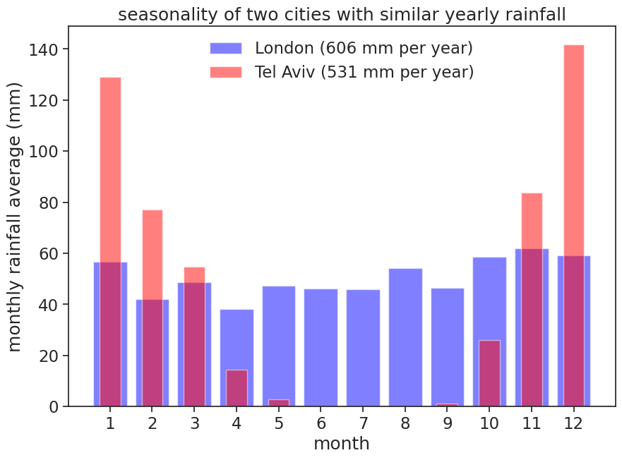
3.1 hydrological year
The hydrological year is time period of 12 months for which precipitation totals are measured. The hydrological year is designated by the calendar year in which it ends.
In temperate regions with distinct seasonal patterns, the hydrological year often starts in the fall, when precipitation and streamflow are typically at their lowest levels. This timing ensures that most of the surface runoff during the water year is attributable to the precipitation that fell during the same period.
Let’s define the hydrological year for Tel Aviv from 1 October to 30 September.
האם אקלים הגשם שלנו משתנה
We will now shift the months according to Tel Aviv’s hydrological year.
plot rainfall distribution according to Tel Aviv’s hydrological year
fig, ax = plt.subplots(figsize=(10,7))
Nroll = 3  # number of months to roll
roll_telaviv = np.roll(monthly_telaviv['PRCP'], Nroll)
roll_london = np.roll(monthly_london['PRCP'], Nroll)
roll_months = np.roll(monthly_london.index, Nroll)
# bar plots
ax.bar(monthly_london.index, roll_london,
        alpha=0.5, color="blue", label=f"London ({monthly_london.values.sum():.0f} mm per year)")
ax.bar(monthly_telaviv.index, roll_telaviv,
        alpha=0.5, color="red", width=0.5, label=f"Tel Aviv ({monthly_telaviv.values.sum():.0f} mm per year)")

# axes labels and figure title
ax.set(xlabel='month',
       ylabel='monthly rainfall average (mm)',
       title='seasonality of two cities with similar yearly rainfall',
       xticks=monthly_london.index,
       xticklabels=roll_months
      )
ax.legend(loc='upper right', frameon=False);

# save figure
# plt.savefig("monthly_tel_aviv_london_bars.png")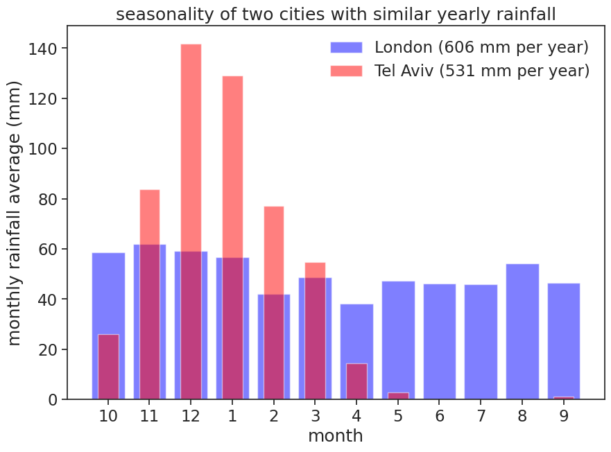
Another way of representing this data is with polar coordinates:
plot in polar coordinates
fig = plt.figure(figsize=(10,10))

# radar chart
ax = fig.add_subplot(111, polar=True)     # make polar plot
ax.set_theta_zero_location("N")           # January on top ("N"orth)
ax.set_theta_direction(-1)                # clockwise direction
ax.set_rlabel_position(90)                # radial labels on the right
ax.set_rticks([50,100])                   # two radial ticks is enough
ax.set_rlim(0,150)                        # limits of r axis
angles=np.linspace(0, 2*np.pi, 12, endpoint=False)       # divide circle into 12 slices
angles=np.append(angles, angles[0])                      # close loop, otherwise lines will be open
month_names = ['Jan', 'Feb', 'Mar', 'Apr', 'May', 'Jun', 'Jul', 'Aug', 'Sep', 'Oct', 'Nov', 'Dec']
ax.set_thetagrids(angles[:-1] * 180/np.pi, month_names)  # relabel angles with month names

# plot london data
stats_london = np.array(monthly_london['PRCP'].values)        # get london data
stats_london = np.append(stats_london, stats_london[0])            # close loop
ax.plot(angles, stats_london, "o-", color='blue', label="london")  # plot line
ax.fill(angles, stats_london, alpha=0.25, color='blue')            # fill

# plot tel aviv data
stats_telaviv = np.array(monthly_telaviv['PRCP'].values)        # get tel aviv data
stats_telaviv = np.append(stats_telaviv, stats_telaviv[0])           # close loop
ax.plot(angles, stats_telaviv, "o-", color='red', label="tel aviv")  # plot line
ax.fill(angles, stats_telaviv, alpha=0.25, color='red')              # fill

ax.set_title("Monthly rainfall averages")
ax.legend(loc=(-0.1,0.9));  # legend at x=-0.2 so it doesn't overlap with graph

# save figure
# plt.savefig("radar_chart_tel_aviv_london.png")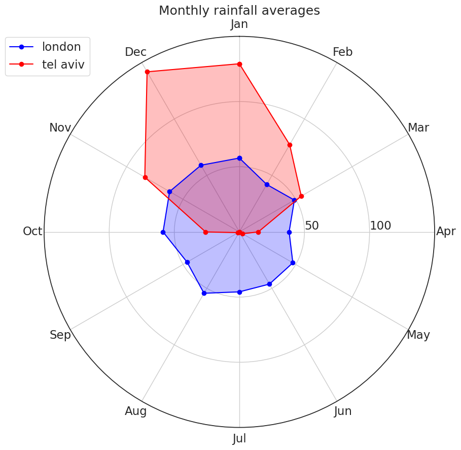
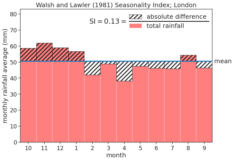
3.2 Seasonality Index
Sources: leddris (2010), Walsh and Lawler (1981)
\langle{P}\rangle= mean annual precipitation
m_i= precipitation mean for month i
SI = \displaystyle \frac{1}{\langle{P}\rangle} \sum_{n=1}^{n=12} \left| m_i - \frac{\langle{P}\rangle}{12} \right|
| SI | Precipitation Regime |
|---|---|
| <0.19 | Precipitation spread throughout the year |
| 0.20-0.39 | Precipitation spread throughout the year, but with a definite wetter season |
| 0.40-0.59 | Rather seasonal with a short dry season |
| 0.60-0.79 | Seasonal |
| 0.80-0.99 | Marked seasonal with a long dry season |
| 1.00-1.19 | Most precipitation in <3 months |
Let’s write some code to calculate the SI for Tel Aviv and London.
Show/hide the code
def walsh_index(df):
    m = df["PRCP"].values
    R = m.sum()
    SI = np.sum(np.abs(m-R/12)) / R
    return SI

london_index = walsh_index(monthly_london)
telaviv_index = walsh_index(monthly_telaviv)
print("Seasonality index (Walsh and Lawler, 1981)")
print(f"London: {london_index:.2f}")
print(f"Tel Aviv: {telaviv_index:.2f}")
Seasonality index (Walsh and Lawler, 1981)
London: 0.13
Tel Aviv: 1.00Show the code
fig, ax = plt.subplots(figsize=(10,7))

plt.rcParams['hatch.linewidth'] = 3
roll_telaviv
xlim = [1, 13]
total_telaviv = np.sum(roll_telaviv)
ax.plot(xlim, [total_telaviv/12]*2, color="tab:blue", linewidth=3)
ax.set_xlim(xlim)

shaded = roll_telaviv - total_telaviv/12
months = monthly_telaviv.index
ax.bar(months, shaded,
       alpha=0.9, color="None", width=1,
       hatch="//", edgecolor='k',
       align='edge', bottom=total_telaviv/12,
       label=f"absolute difference")

ax.bar(months, roll_telaviv,
       alpha=0.5, color="red", width=1,
       align='edge',
       label=f"total rainfall", zorder=0)

ax.text(5.3, 86.5, r"SI$=1.00=$", fontsize=20)
ax.text(xlim[-1], total_telaviv/12, " mean", va="center")
ax.plot([7.8, 12.8], [89.5]*2, color="black", lw=2)
# axes labels and figure title
ax.set(xlabel='month',
       ylabel='monthly rainfall average (mm)',
       title='Walsh and Lawler (1981) Seasonality Index; Tel Aviv',
       xticks=np.arange(1.5,12.6,1),
       xticklabels=roll_months,
      )

plt.legend(loc='upper right', frameon=False, bbox_to_anchor=(1, 0.7),
           fontsize=18);

# save figure
# plt.savefig("si_walsh_telaviv.png")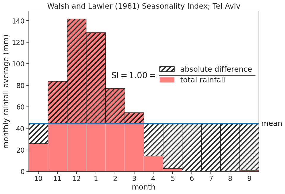
Show the code
fig, ax = plt.subplots(figsize=(10,7))

plt.rcParams['hatch.linewidth'] = 3
xlim = [1, 13]
total_london = np.sum(roll_london)
ax.plot(xlim, [total_london/12]*2, color="tab:blue", linewidth=3)
ax.set_xlim(xlim)

shaded = roll_london - total_london/12
months = monthly_london.index
ax.bar(months, shaded,
       alpha=0.9, color="None", width=1,
       hatch="//", edgecolor='k',
       align='edge', bottom=total_london/12,
       label=f"absolute difference")

ax.bar(months, roll_london,
       alpha=0.5, color="red", width=1,
       align='edge',
       label=f"total rainfall", zorder=0)


ax.text(5.3, 74, r"SI$=0.13=$", fontsize=20)
ax.text(xlim[-1], total_london/12, " mean", va="center")
ax.plot([7.8, 12.8], [75.5]*2, color="black", lw=2)
# axes labels and figure title
ax.set(xlabel='month',
       ylabel='monthly rainfall average (mm)',
       title='Walsh and Lawler (1981) Seasonality Index; London',
       xticks=np.arange(1.5,12.6,1),
       xticklabels=roll_months,
       ylim=[0,83],
      )

plt.legend(loc='upper right', frameon=False, bbox_to_anchor=(1, 1.005),
           fontsize=18);

# save figure
# plt.savefig("si_walsh_telaviv.png")