The group SL(2) is the group of 2x2 matrices with determinant 1. It is a fundamental example in the study of Lie groups and Lie algebras. The determinant of a matrix measures volume scaling. If you apply a linear transformation with matrix A to a region of space, the volume gets multiplied by \det(A). So \det=1 means volume preserving transformations. This is a very natural class of symmetries — transformations that don’t shrink or expand space, just reshape it.
Play with the widget below and and get a feel for three kinds of transformations that preserve area in 2d space: rotation, shear, and squish/stretch. The last panel shows all three operations at once.
A general element of this group can be written as:
g = \begin{pmatrix} a & b \\ c & d \end{pmatrix}
where a, b, c, d \in \mathbb{C} and the determinant is 1, i.e., ad - bc = 1.
Change of point of view. Each of the elements a,b,c,d is complex-valued, and we can imagine that every matrix in SL(2,\mathbb{C}) is a point in an 4-dimensional complex space \mathbb{C}^4 . However, the constraint that the determinant equals 1 reduces the degrees of freedom by 1, meaning that the group SL(2,\mathbb{C}) is a 3-dimensional surface embedded in a larger \mathbb{C}^4 space. (If you prefer to think of 1 complex dimension as equivalent to 2 real dimensions, then just multiply all the dimensions by 2.) This surface is curved, because of the nonlinear constraint ad - bc = 1. In mathematical parlance, we call this surface a manifold.
13.2 tangent space
Let’s parametrize each element of the 2\times2 matrix in SL(2) with the variable t:
We can imagine that this parametrization defines a general curve in the manifold of SL(2). We will require that this curve passes through the identity element of SL(2) at t = 0:
What we will do now is to take the derivative of this curve with respect to the parameter t, which will give us a vector in the tangent space of SL(2) at each point:
\dot{g}(t) = \begin{pmatrix} \dot{a}(t) & \dot{b}(t) \\ \dot{c}(t) & \dot{d}(t) \end{pmatrix},
where the dot means “time derivative”.
We are particularly interested in the tangent space at the identity, so we evaluate the vector \dot{g} at t=0, and we’ll call it X for simplicity’s sake:
Now let’s see how the constraint that an element g in SL(2) has a determinant equal to 1 translates into this tangent vector X. For that, we compute the derivative of the condition ad - bc = 1 with respect to t, and evaluate it at t = 0:
This means that, in the same way that the element g of the group has dimension 3, it’s tangent vector at the identity X also has dimension 3.
Let’s take stock of what happened. From Calculus (and Physics), we are used to the idea that taking the time-derivative of the position curve gives us a vector for the velocity. The velocity is tangent to the displacement curve at each point. That’s exactly what we did here, but we did it for all possible curves in the manifold that pass through the identity element of SL(2). By taking the derivative of the curves A(t) at t = 0 (at the identity element), we obtained vectors in the tangent space of SL(2) at that point. These new vectors have exactly the same dimension as the original (in this case 3 complex dimensions), but they live in a flat (Euclidean) space rather than in the curved manifold of SL(2).
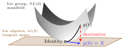
The curved gray surface represents the manifold of SL(2), and the plane below it represents the tangent space at the identity element. The curve g(t) in the manifold passes through the identity, and its derivative at that point is the blue tangent vector X.
13.3 back and forth between the group and the tangent space
We’ve seen that, starting from a curve g(t), we can get to an element of the tangent space X by taking its derivative at the identity:
g(t) \xrightarrow[]{\frac{d}{dt}} X.
How do we go back? Starting from X in the tangent space, how to get the curve g in the manifold? The answer is: exponentiation!
X \xrightarrow[]{\exp} g(t).
Let’s see how this works. X is a 2\times2 matrix, and its (parametric) exponential is
This is exactly the same formula for the exponent of scalars, but applied to matrices. Note that the identity matrix I takes the role of the number 1. The matrix X raised to any power is still a 2\times2 matrix. Therefore, the series above also gives as a result a 2\times2 matrix. Now, how can we know if this new matrix “lands” in the manifold, where the group elements live? We just need to check if the determinant of \exp(tX) is 1, if it is, we’re golden.
And this shows that exponentiating an element of the tangent space brings us to a curve g(t) in the manifold.
The proof is water tight, but somewhat not satisfying. I guessed that the solution was the exponential, and verified that it does the job. Why should the exponential appear in the first place?
The previous analogy between position and velocity will be useful. If a particle has position x(t) and constant velocity v, then for a very small time step \Delta t
v \approx \frac{x(t+\Delta t)-x(t)}{\Delta t}.
Rearranging,
x(t+\Delta t) \approx x(t) + \Delta t \cdot v.
So in ordinary Euclidean space, constant velocity means that each small time step updates the position by
x(t)\longmapsto x(t)+\Delta t\cdot v
The same idea works for a Lie group, except that the update operation is no longer addition. In a group, motions are composed by multiplication. Therefore, the analogue of adding a small displacement is multiplying by a small group element near the identity.
If g(t) is a curve in the manifold for which g(0)=I and \dot{g}(0)=X, we can rewrite its derivative by using the definition
We’ve reached the same result as before, but this time the exponential appears naturally from the derivation.
To sum up: taking the derivative of a curve g(t) in the manifold gives us the element X in the tangent space. Exponentiating X brings us back to g(t).
13.4 wait, what?
Is this correct? The derivative and the exponential are lanes travelling in opposite directions in the same road? Usually, we have the following pairs: (\exp,\log) and (\text{derivative},\text{integral}). Did we not just mix elements of these two pairs?
I will show now that, in a sense, taking the derivative or the log of a group element is the same. Conversely, exponentiating or integrating an element in the tangent space give the same result.
13.4.1 derivative = log
Let’s take a group element g close to the identity. We can write it as
g = I + \Delta t X + O(\Delta t^2),
where X is some matrix and \Delta t is small. Taking the log:
\log(g) = \log(I + \Delta t X + O(\Delta t^2)).
We now use the Taylor series for the log:
\begin{align}
\log(g) &= \log(I+\Delta t X) \\
&= \Delta t X - \frac{(\Delta t X)^2}{2} + \frac{(\Delta t X)^3}{3} - \ldots \\
&= \Delta t X + O(\Delta t^2).
\end{align}
To leading order in \Delta t, the log simply gives back \Delta t X, which is exactly the tangent vector X, up to the small parameter \Delta t.
Both the derivative and the log do the same job, they extract the linear part of the deviation from the identity. Differentiation gives the exact geometric definition for what the tangent space is, while the logarithm is a computational shortcut, it extracts the tangent vector from a specific point near the identity, without needing a whole curve in the manifold.
13.4.2 integral = exp
We’ve seen before that the rule for taking small steps along a curve g(t) is
It says that g(t) is not any curve on the manifold that passes through the identity. This is the one curve whose velocity at any point is proportional to itself!
Of course, we can solve this first-order differential equation by integrating it, giving what we found before: g(t)=\exp(tX). Thus we have shown that, in a sense, integration and exponentiation give the same thing.
13.5 the tangent space is a vector space
A vector space has the following property: if A and B are two vectors in the vector space, their linear combination \mu_1 A + \mu_2 B is also a vector belonging to this vector space. The one condition we know about the tangent space is that its elements are 2\times2 matrices with trace zero. So let’s use that to prove that our tangent space is a vector space. Using the fact that the trace operation is linear:
\text{trace}(\mu_1 A + \mu_2 B) = \mu_1 \underbrace{\text{trace}(A)}_{=0} + \mu_2 \underbrace{\text{trace}(B)}_{=0} = 0.
If you want to see this in extra detail, let’s write
An algebra is a vector space equipped with a special operation. The natural operation of vector spaces is the addition: you can add two vectors and get another vector. That’s not what I’m talking about. The extra operation also takes two vectors and return a third vector. What should this extra operation be? The answer is related to a concept we have not discussed yet: commutativity
13.7 commutativity
Putting one’s socks on, and then the shoes, is not the same as putting the shoes on and then the socks. The order of operations often matters.
When the order of two operations doesn’t affect the result, we say that the operations commute. Simple examples are the sum and product of two numbers
Maybe you’re thinking: “There are not two operations in the example above, there is only one sum and one product, one for each example! The numbers commute, not the operations!” Sure, this is a legitimate way of seeing things. Another way is to, in the summation example, see every number as its own summation operation, being applied on a “test element” x not shown. Let me spell out how this looks:
+3+5+x = +5+3+x = +8+x.
The same goes for the product: 2\cdot 7\cdot x = 7\cdot 2\cdot x.
13.8 non-commutativity
Of course, non-commutativity is the name we give to operations whose order does affect the result. I’ll give a concrete example here using rotations, and it turns out that this will be super useful to us. Rotations in 3d space are a special case inside the bigger Lie group SL(2). I’ll use rotations because this is something we have lots of intuition about from day-to-day experience.
We will talk about rotation using the image of Earth. See the widget below.
On the left we see Earth with a head-on view of the equator, centered at the meridian 75E, making India right at the center.
On the center we can slide the slider labeled g(t), to spin Earth to the right (eastward), so that by the end of the slider Earth has rotated 75 degrees, and now we see the zero meridian at Greenwich at the center.
On the right we can slide the slider labeled k(t), to tilt Earth counter-clockwise on the plane of the screen where you’re seeing this image, so that by the end of the slider Earth has tilted 23.44 degrees.
The question now is: does the order or operations matter? Spinning to the right and then tilting is the same as the opposite order? Let’s see this in action. In the widget below:
On the globe on the left, first slide g(t) on the top and then k(t) at the bottom.
On the globe on the right, slide first k(t) and then g(t).
Show the code
{const W=280, H=340, R=115, cx=W/2, cy=165, ext=40, gap=20;const BG='#dddddd', OCEAN='#84a1b7', π=Math.PI;// ── explicit 3×3 rotation matrices in the fixed observer frame ────────────// screen/view convention:// x = viewing direction, y = screen horizontal, z = screen vertical//// a = Rz: eastward rotation around the fixed screen-vertical axis// b = Rx: tilt/roll around the fixed viewing axis, so the pole tilts in screen planefunctionRz(deg) {const c=Math.cos(deg*π/180), s=Math.sin(deg*π/180);return [[c,-s,0],[s,c,0],[0,0,1]]; }functionRx(deg) {const c=Math.cos(deg*π/180), s=Math.sin(deg*π/180);return [[1,0,0],[0,c,-s],[0,s,c]]; }functionmul(A,B) {const C=[[0,0,0],[0,0,0],[0,0,0]];for(let i=0;i<3;i++) for(let j=0;j<3;j++) for(let k=0;k<3;k++) C[i][j]+=A[i][k]*B[k][j];return C; }functionapplyM(M, lon, lat) {const φ=lat*π/180, λ=lon*π/180;const x=Math.cos(φ)*Math.cos(λ);const y=Math.cos(φ)*Math.sin(λ);const z=Math.sin(φ);const rx=M[0][0]*x+M[0][1]*y+M[0][2]*z;const ry=M[1][0]*x+M[1][1]*y+M[1][2]*z;const rz=M[2][0]*x+M[2][1]*y+M[2][2]*z;return [Math.atan2(ry,rx)*180/π,Math.asin(Math.max(-1,Math.min(1,rz)))*180/π ]; }const INIT =Rz(-75);functionmakeSlider(label, min, max, step, init) {const wrap=document.createElement('div'); wrap.style.cssText='margin-bottom:5px';const lbl=document.createElement('label'); lbl.textContent=label; lbl.style.cssText='color:black;font-family:Arial,sans-serif;font-size:13px;'+'font-weight:bold;display:block;margin-bottom:1px';const inp=document.createElement('input'); inp.type='range'; inp.min=min; inp.max=max; inp.step=step; inp.value=init; inp.style.cssText='width:100%;display:block;cursor:pointer;margin:0'; wrap.append(lbl,inp);return {wrap,inp}; }const {wrap:wLA,inp:iLA}=makeSlider('g(t)',0,75,1,0);const {wrap:wLB,inp:iLB}=makeSlider('k(t)',0,23.44,0.1,0);const {wrap:wRB,inp:iRB}=makeSlider('k(t)',0,23.44,0.1,0);const {wrap:wRA,inp:iRA}=makeSlider('g(t)',0,75,1,0);const container=document.createElement('div'); container.style.cssText=`background:${BG};padding:8px;display:flex;`+`gap:${gap}px;width:${2*W+gap+16}px;box-sizing:border-box;align-items:flex-start`;const colL=document.createElement('div'); colL.style.cssText=`width:${W}px;flex-shrink:0`;const svgL=d3.create('svg').attr('width',W).attr('height',H).style('background',BG).node(); colL.append(wLA,wLB,svgL);const colR=document.createElement('div'); colR.style.cssText=`width:${W}px;flex-shrink:0`;const svgR=d3.create('svg').attr('width',W).attr('height',H).style('background',BG).node(); colR.append(wRB,wRA,svgR); container.append(colL,colR);functiondraw(svgNode, M) {const svg=d3.select(svgNode); svg.selectAll('*').remove();const fn=(lon,lat)=>applyM(M,lon,lat);const baseProj=d3.geoOrthographic().scale(R).translate([cx,cy]).rotate([0,0,0]);const customProj={stream(sink){const ps=baseProj.stream(sink);return {point(lon,lat){const [rl,rp]=fn(lon,lat); ps.point(rl,rp); },lineStart(){ ps.lineStart(); },lineEnd(){ ps.lineEnd(); },polygonStart(){ ps.polygonStart(); },polygonEnd(){ ps.polygonEnd(); },sphere(){ if(ps.sphere) ps.sphere(); } }; } };const path=d3.geoPath(customProj);functionproject(lon,lat){const [rl,rp]=fn(lon,lat);returnbaseProj([rl,rp]); }const npPx=project(0,90)??[cx,cy-R];const spPx=project(0,-90)??[cx,cy+R];const dx=npPx[0]-spPx[0];const dy=npPx[1]-spPx[1];const len=Math.sqrt(dx*dx+dy*dy)||1;const ux=dx/len;const uy=dy/len;const poleDepth=M[0][2];const eps=0.01;functiondrawAxisSegment(parent, polePx, sign) {const tx=polePx[0]+sign*ux*ext;const ty=polePx[1]+sign*uy*ext; parent.append('line').attr('x1',polePx[0]).attr('y1',polePx[1]).attr('x2',tx).attr('y2',ty).attr('stroke','#e17701').attr('stroke-width',2.5); parent.append('circle').attr('cx',tx).attr('cy',ty).attr('r',3.5).attr('fill','#e17701'); }// draw the back-facing axis segment first, so the globe occludes itif(poleDepth > eps){drawAxisSegment(svg, spPx,-1); } elseif(poleDepth <-eps){drawAxisSegment(svg, npPx,1); } svg.append('circle').attr('cx',cx).attr('cy',cy).attr('r',R).attr('fill',OCEAN); svg.append('path').datum(d3.geoGraticule().step([15,90])()).attr('fill','none').attr('stroke','rgba(200,200,200,0.40)').attr('stroke-width',0.7).attr('d',path); svg.append('path').datum({type:'LineString',coordinates:d3.range(-180,181,1).map(l=>[l,0])}).attr('fill','none').attr('stroke','rgba(255,255,180,0.35)').attr('stroke-width',1).attr('d',path); svg.append('path').datum(topojson.feature(world,world.objects.land)).attr('fill','#2d6a1f').attr('d',path); svg.append('path').datum(topojson.mesh(world,world.objects.countries)).attr('fill','none').attr('stroke','rgba(255,255,255,0.35)').attr('stroke-width',0.5).attr('d',path); svg.append('circle').attr('cx',cx).attr('cy',cy).attr('r',R).attr('fill','none').attr('stroke','rgba(0,0,0,0.20)').attr('stroke-width',1);// draw the front-facing axis segment last, so it appears to emerge from the globeif(poleDepth > eps){drawAxisSegment(svg, npPx,1); } elseif(poleDepth <-eps){drawAxisSegment(svg, spPx,-1); } else {drawAxisSegment(svg, npPx,1);drawAxisSegment(svg, spPx,-1); }}// ── stateful ambient-frame updates ────────────────────────────────────────//// important:// slider values are not recomputed into a fresh matrix.// instead, each slider movement applies the delta since the previous value.// this preserves the historical order in which the user moved the sliders.const stateL = {M: INIT,A:+iLA.value,B:+iLB.value };const stateR = {M: INIT,A:+iRA.value,B:+iRB.value };functionredraw(){draw(svgL,stateL.M);draw(svgR,stateR.M); } iLA.addEventListener('input',() => {const next=+iLA.value;const delta=next-stateL.A; stateL.M=mul(Rz(delta),stateL.M); stateL.A=next;redraw(); }); iLB.addEventListener('input',() => {const next=+iLB.value;const delta=next-stateL.B; stateL.M=mul(Rx(delta),stateL.M); stateL.B=next;redraw(); }); iRA.addEventListener('input',() => {const next=+iRA.value;const delta=next-stateR.A; stateR.M=mul(Rz(delta),stateR.M); stateR.A=next;redraw(); }); iRB.addEventListener('input',() => {const next=+iRB.value;const delta=next-stateR.B; stateR.M=mul(Rx(delta),stateR.M); stateR.B=next;redraw(); });redraw();return container;}
Did you get the same thing? No! If you think there’s something suspicious with this simulations, just take any object around you and try it yourself. I recomment doing 90-degree rotations because it’s just easier to keep track of what’s going on. One more thing: the operation g(t) means spinning the globe to the right, no matter where the plane of the equator is. That is to say that the operations are with respect to an external coordinate system (the screen where you’re reading this), not the globe’s own coordinate system.
The conclusion: the order of operation matters when we’re dealing with rotations.
13.9 quantifying the non-commutativity
Ok, the order of operation matters, but how much? Is the difference barely perceptible, or super consequential? How to quantify it? We are wondering, “is gk equal to kg?”
gk \stackrel{?}{=} kg
In order to find the difference between the two sides of the equation, ideally I would subtract the same quantity from both sides. Unfortunately, groups only have multiplication and the inverse, not addition/subtraction. To measure the effect of doing operations in different orders, we right-multiply both sides of the equation by g^{-1} and then right-multiply again by k^{-1}. We get:
gkg^{-1}k^{-1} \stackrel{?}{=} I.
Conjugations of group operations are read right-to-left, so the left-hand side above, called group commutator, says: “apply k^{-1}, then g^{-1}, then k and finally g. The question mark on top of the equal sign is asking:”if we did all that, would the final result bring us back home, to our starting place?”
Let’s see that in action with globe rotations. Slide each of the sliders from top to bottom and see if the result equals to the unchanged globe on the right.
Show the code
{const W=280, H=340, R=115, cx=W/2, cy=165, ext=40, gap=20;const BG='#dddddd', OCEAN='#84a1b7', π=Math.PI;// ── explicit 3×3 rotation matrices in the fixed observer frame ────────────// screen/view convention:// x = viewing direction, y = screen horizontal, z = screen vertical//// g = Rz: eastward rotation around the fixed screen-vertical axis// k = Rx: tilt/roll around the fixed viewing axis, so the pole tilts in screen planefunctionRz(deg) {const c=Math.cos(deg*π/180), s=Math.sin(deg*π/180);return [[c,-s,0],[s,c,0],[0,0,1]]; }functionRx(deg) {const c=Math.cos(deg*π/180), s=Math.sin(deg*π/180);return [[1,0,0],[0,c,-s],[0,s,c]]; }functionmul(A,B) {const C=[[0,0,0],[0,0,0],[0,0,0]];for(let i=0;i<3;i++) for(let j=0;j<3;j++) for(let k=0;k<3;k++) C[i][j]+=A[i][k]*B[k][j];return C; }functionapplyM(M, lon, lat) {const φ=lat*π/180, λ=lon*π/180;const x=Math.cos(φ)*Math.cos(λ);const y=Math.cos(φ)*Math.sin(λ);const z=Math.sin(φ);const rx=M[0][0]*x+M[0][1]*y+M[0][2]*z;const ry=M[1][0]*x+M[1][1]*y+M[1][2]*z;const rz=M[2][0]*x+M[2][1]*y+M[2][2]*z;return [Math.atan2(ry,rx)*180/π,Math.asin(Math.max(-1,Math.min(1,rz)))*180/π ]; }const INIT =Rz(-75);functionmakeSlider(label, min, max, step, init) {const wrap=document.createElement('div'); wrap.style.cssText='margin-bottom:5px';const lbl=document.createElement('label'); lbl.innerHTML=label; lbl.style.cssText='color:black;font-family:Arial,sans-serif;font-size:13px;'+'font-weight:bold;display:block;margin-bottom:1px';const inp=document.createElement('input'); inp.type='range'; inp.min=min; inp.max=max; inp.step=step; inp.value=init; inp.style.cssText='width:100%;display:block;cursor:pointer;margin:0'; wrap.append(lbl,inp);return {wrap,inp}; }functionmakeHiddenSliderSpacer(label, min, max, step, init) {const {wrap}=makeSlider(label, min, max, step, init); wrap.style.visibility='hidden'; wrap.style.pointerEvents='none';return wrap; }const {wrap:wLKi,inp:iLKi}=makeSlider('k<sup>−1</sup>(t)',0,23.44,0.1,0);const {wrap:wLGi,inp:iLGi}=makeSlider('g<sup>−1</sup>(t)',0,75,1,0);const {wrap:wLK,inp:iLK}=makeSlider('k(t)',0,23.44,0.1,0);const {wrap:wLG,inp:iLG}=makeSlider('g(t)',0,75,1,0);const container=document.createElement('div'); container.style.cssText=`background:${BG};padding:8px;display:flex;`+`gap:${gap}px;width:${2*W+gap+16}px;box-sizing:border-box;align-items:flex-start`;const colL=document.createElement('div'); colL.style.cssText=`width:${W}px;flex-shrink:0`;const svgL=d3.create('svg').attr('width',W).attr('height',H).style('background',BG).node(); colL.append(wLKi,wLGi,wLK,wLG,svgL);const colR=document.createElement('div'); colR.style.cssText=`width:${W}px;flex-shrink:0`;const svgR=d3.create('svg').attr('width',W).attr('height',H).style('background',BG).node(); colR.append(makeHiddenSliderSpacer('k<sup>−1</sup>(t)',0,23.44,0.1,0),makeHiddenSliderSpacer('g<sup>−1</sup>(t)',0,75,1,0),makeHiddenSliderSpacer('k(t)',0,23.44,0.1,0),makeHiddenSliderSpacer('g(t)',0,75,1,0), svgR ); container.append(colL,colR);functiondraw(svgNode, M) {const svg=d3.select(svgNode); svg.selectAll('*').remove();const fn=(lon,lat)=>applyM(M,lon,lat);const baseProj=d3.geoOrthographic().scale(R).translate([cx,cy]).rotate([0,0,0]);const customProj={stream(sink){const ps=baseProj.stream(sink);return {point(lon,lat){const [rl,rp]=fn(lon,lat); ps.point(rl,rp); },lineStart(){ ps.lineStart(); },lineEnd(){ ps.lineEnd(); },polygonStart(){ ps.polygonStart(); },polygonEnd(){ ps.polygonEnd(); },sphere(){ if(ps.sphere) ps.sphere(); } }; } };const path=d3.geoPath(customProj);functionproject(lon,lat){const [rl,rp]=fn(lon,lat);returnbaseProj([rl,rp]); }const npPx=project(0,90)??[cx,cy-R];const spPx=project(0,-90)??[cx,cy+R];const dx=npPx[0]-spPx[0];const dy=npPx[1]-spPx[1];const len=Math.sqrt(dx*dx+dy*dy)||1;const ux=dx/len;const uy=dy/len;const poleDepth=M[0][2];const eps=0.01;functiondrawAxisSegment(parent, polePx, sign) {const tx=polePx[0]+sign*ux*ext;const ty=polePx[1]+sign*uy*ext; parent.append('line').attr('x1',polePx[0]).attr('y1',polePx[1]).attr('x2',tx).attr('y2',ty).attr('stroke','#e17701').attr('stroke-width',2.5); parent.append('circle').attr('cx',tx).attr('cy',ty).attr('r',3.5).attr('fill','#e17701'); }// draw the back-facing axis segment first, so the globe occludes itif(poleDepth > eps){drawAxisSegment(svg, spPx,-1); } elseif(poleDepth <-eps){drawAxisSegment(svg, npPx,1); } svg.append('circle').attr('cx',cx).attr('cy',cy).attr('r',R).attr('fill',OCEAN); svg.append('path').datum(d3.geoGraticule().step([15,90])()).attr('fill','none').attr('stroke','rgba(200,200,200,0.40)').attr('stroke-width',0.7).attr('d',path); svg.append('path').datum({type:'LineString',coordinates:d3.range(-180,181,1).map(l=>[l,0])}).attr('fill','none').attr('stroke','rgba(255,255,180,0.35)').attr('stroke-width',1).attr('d',path); svg.append('path').datum(topojson.feature(world,world.objects.land)).attr('fill','#2d6a1f').attr('d',path); svg.append('path').datum(topojson.mesh(world,world.objects.countries)).attr('fill','none').attr('stroke','rgba(255,255,255,0.35)').attr('stroke-width',0.5).attr('d',path); svg.append('circle').attr('cx',cx).attr('cy',cy).attr('r',R).attr('fill','none').attr('stroke','rgba(0,0,0,0.20)').attr('stroke-width',1);// draw the front-facing axis segment last, so it appears to emerge from the globeif(poleDepth > eps){drawAxisSegment(svg, npPx,1); } elseif(poleDepth <-eps){drawAxisSegment(svg, spPx,-1); } else {drawAxisSegment(svg, npPx,1);drawAxisSegment(svg, spPx,-1); } }// ── stateful ambient-frame updates ────────────────────────────────────────//// important:// slider values are not recomputed into a fresh matrix.// instead, each slider movement applies the delta since the previous value.// this preserves the historical order in which the user moved the sliders.const stateL = {M: INIT,Ki:+iLKi.value,Gi:+iLGi.value,K:+iLK.value,G:+iLG.value };functionredraw(){draw(svgL,stateL.M);draw(svgR,INIT); } iLKi.addEventListener('input',() => {const next=+iLKi.value;const delta=next-stateL.Ki; stateL.M=mul(Rx(-delta),stateL.M); stateL.Ki=next;redraw(); }); iLGi.addEventListener('input',() => {const next=+iLGi.value;const delta=next-stateL.Gi; stateL.M=mul(Rz(-delta),stateL.M); stateL.Gi=next;redraw(); }); iLK.addEventListener('input',() => {const next=+iLK.value;const delta=next-stateL.K; stateL.M=mul(Rx(delta),stateL.M); stateL.K=next;redraw(); }); iLG.addEventListener('input',() => {const next=+iLG.value;const delta=next-stateL.G; stateL.M=mul(Rz(delta),stateL.M); stateL.G=next;redraw(); });redraw();return container;}
Now it’s time to quantify by how much the result we got on the left if different from that on the right. The sliders g and k applied rotations of 75 and 23.44 degrees, respectively. We will quantify the group commutator by taking infinitesimal rotations. Taking advantage of the fact that we can express group elements and the exponentiation of the tangent space elements, we will write
g = \exp(\epsilon A),\qquad k = \exp(\epsilon B),
where \epsilon is a small parameter. If g(t)=\exp(tA), then think of g = \exp(\epsilon A) as leaving from the identity and following the curve g(t) for a very small time interval \epsilon. The group commutator then reads
\begin{align*}
gkg^{-1}k^{-1} =& e^{\epsilon A}e^{\epsilon B}e^{-\epsilon A}e^{-\epsilon B} \\
=& (I + \epsilon A + \tfrac{\epsilon^2}{2} A^2 \ldots) \\
\times & (I + \epsilon B + \tfrac{\epsilon^2}{2} B^2 \ldots) \\
\times & (I - \epsilon A + \tfrac{\epsilon^2}{2} A^2 \ldots) \\
\times & (I - \epsilon B + \tfrac{\epsilon^2}{2} B^2 \ldots) \\
=& \\
\text{order }\epsilon^0:&\quad I + \\
\text{order }\epsilon^1:&\quad \epsilon(A+B-A-B) + \\
\text{order }\epsilon^2:&\quad \epsilon^2(AB-A^2-AB-BA-B^2+AB + \\
&\quad \phantom{\epsilon^2(}\tfrac{\epsilon^2}{2} A^2+\tfrac{\epsilon^2}{2} B^2+\tfrac{\epsilon^2}{2} A^2+\tfrac{\epsilon^2}{2} B^2 )\\
&+\text{ higher order terms in }\epsilon
\end{align*}
All the terms in order \epsilon^1 cancel out, and many of the terms in order \epsilon^2 cancel out too, but not all. The result is:
gkg^{-1}k^{-1} = I + \epsilon^2\left(AB-BA\right) + O(\epsilon^3)
So now we can answer our question: how different is the group commutator from the identity? The difference is small, but not zero. There are no terms of order \epsilon, while the terms of order \epsilon^2 give a nice expression, AB-BA. Because A and B are elements of the algebra, we call this the algebra commutator, and we express it with the square brackets [A,B], called Lie brackets.
Now that we are somewhat familiar with the algebra commutator, we can discuss explicitly what it means for the tangent space to be “an algebra”. We showed that the tangent space is a vector space. This is the first requirement. The second, is that this vector space is equipped with an extra operator that takes two elements in the vector space and returns another element in the space. This special operator is the Lie bracket [A,B]=AB-BA. Lastly, we need to show that this operator satisfies the following properties: closure, bilinearity, antisymmetry, and the Jacobi identity. Let’s go through each of these properties one by one.
13.11 closure
Closure means that if we take two elements in the tangent space, A and B, and apply the Lie bracket to them, the result is also an element in the tangent space. In other words, if A and B are both 2\times 2 matrices with trace zero, then [A,B] is also a 2\times 2 matrix with trace zero. This is important because it ensures that the Lie bracket operation does not take us out of the tangent space.
Let’s take two arbitrary elements in the tangent space, A and B, and compute their Lie bracket:
and it is easy to see now that the trace of [A,B] is zero. This proves that the Lie bracket is closed in the tangent space.
13.12 bilinearity
Bilinearity means that the Lie bracket is linear in both of its arguments. In other words, if we take two elements in the tangent space, A and B, and a scalar \alpha, then we have:
This property is important because it allows us to scale the elements in the tangent space and still have the Lie bracket behave in a predictable way.
13.13 antisymmetry
Antisymmetry means that the Lie bracket is antisymmetric in its arguments. In other words, if we take two elements in the tangent space, A and B, then we have:
[A,B] = -[B,A].
Again, we can prove this by expanding the Lie bracket using the definition [A,B] = AB - BA:
[A,B] = AB - BA = -(BA - AB) = -[B,A].
This means that the bracket measures non-commutativity and nothing else — swap the inputs and you flip the sign, with no leftover symmetric part.
13.14 Jacobi identity
The Jacobi identity is a property that relates the Lie bracket of three elements in the tangent space. It states that for any three elements A, B, and C in the tangent space, we have:
[A,[B,C]] + [B,[C,A]] + [C,[A,B]] = 0.
I will first show that this is true. You will not be satisfied, because this equation seems to have fallen from the sky. Don’t worry, I will soon show you where it comes from. Let’s expand each of the three terms in the Jacobi identity:
You can do the boring task of verifying that when you add all three terms together, everything cancels out and you get zero. This proves the Jacobi identity.
I feel deeply unsatisfied with this proof, because it seems like the Jacobi identity is just a random fact about operators. Let’s see where this comes from.
13.15 group conjugation and the Jacobi identity
If g and k are elements of a group, then the conjugation of k by g is defined as:
gkg^{-1}.
In intuitive terms, the group conjugation gkg^{-1} expresses the operation of applying just k, but in a different frame of reference. By multiplying k on both sides by g and g^{-1}, we have effectively applied k in the frame of reference defined by g. Importantly here, conjugation preserves the bracket structure:
We will now see what happens if we take the group element to be g=\exp(tX), and we take the derivative of the bracket conjugation above with respect to t at t=0. This is similar to what we did in the previous section, where we took the derivative of the group commutator at t=0 to get the algebra commutator. We do this to see how the group conjugation behaves in the tangent space. Taking the derivative of the left-hand side with respect to t at t=0, we have:
Now let’s take the derivative of the right-hand side with respect to t at t=0. For convenience, let’s call \hat{Y} and \hat{Z} the conjugation of Y and Z respectively. We have:
We also note that at t=0, \hat{Y}(0) = e^{0X}Ye^{-0X}=Y and \hat{Z}(0) = e^{0X}Ze^{-0X} = Z. Then continuing with the derivative of the right-hand side, we have:
Substituting these and rearranging, we get the Jacobi identity
[X,[Y,Z]] +[Y,[Z,X]] + [Z,[X,Y]] =0.
The Jacobi identity is a direct consequence of the properties of the group conjugation and the Lie bracket. Specifically, because we applied the product rule to the derivative of the right-hand side, we see that the Jacobi identity is a consequence of the Leibniz rule for derivatives. We will see later in the “adjoint representation” section a very nice connection to this last statement.
13.16 taking stock of what we know
Let’s give formal names to objects we’ve been dealing with.
SL(2) is the group of 2\times 2 matrices with complex elements and determinant 1.
The Lie algebra associated with \mathrm{SL}(2,\mathbb C) is denoted \mathfrak{sl}(2,\mathbb C). It is the tangent space to \mathrm{SL}(2,\mathbb C) at the identity. Its elements are the infinitesimal motions that start at I and remain inside the group, at least to first order.
Concretely,
\mathfrak{sl}(2,\mathbb C)
=
\left\{
X=
\begin{pmatrix}
a&b\\
c&-a
\end{pmatrix}
:
a,b,c\in\mathbb C.
\right\}.
This is why \mathfrak{sl}(2,\mathbb C) is 3-dimensional: it has three free parameters, a,b,c.
The algebra also has its own version of a commutator. If X,Y\in\mathfrak{sl}(2,\mathbb C), we define
[X,Y]=XY-YX.
This is called the Lie bracket. It measures the infinitesimal failure of commutativity.
13.17 a basis for \mathfrak{sl}(2)
Since all elements in the \mathfrak{sl}(2) algebra live in a 3-dimensional vector space, we can define a convenient basis for this space made of three basis elements:
E = \begin{pmatrix}0&1\\0&0\end{pmatrix},\quad
H = \begin{pmatrix}1&0\\0&-1\end{pmatrix},\quad
F = \begin{pmatrix}0&0\\1&0\end{pmatrix}
All three vectors are traceless, and any element in the algebra can be thought of as a linear combination of them:
The linear combination above shows how these elements behave under the basic operation of a vector space: addtion. What about the special operation we defined for the \mathfrak{sl}(2) algebra? How will these basis elements commute? Let’s apply the Lie bracket to each pair of basis vectors and see.
\begin{align*}
[H,E] &= 2E \\
[H,F] &= -2F \\
[E,F] &= H
\end{align*}
You know these commutation relationships are important, because I put them in a box!
13.18 representations
Remember the operations in the very first widget in this page. We had a square, and we could spin in, shear it, or squish/stretch it. All these maintain the area, and mathematically this is enforced by the requirement that the determinant of elements in the group SL(2) equals one.
Rotations, shear and squish/stretch are abstract concepts, and they only get embodied in a specific form once we define on which kind of objects they are operating on. Take rotations, for example. If we are talking about rotating an object in 2d space, this is accomplished by a 2\times 2 matrix. If, instead, we wish to rotate an object in 3d space, that matrix won’t do, we’ll need a 3\times3 matrix to do it. The abstract notion of “rotation” needs to be represented by different things depending on the object it operates on.
So far we’ve started to get to know the group SL(2) and its tangent algebra \mathfrak{sl}(2), and now it’s time to get acquainted with some of its most important representations.
Both groups and algebras have representations, but in what follows we will deal with representation of the algebra. Let me try to justify why this makes sense. A representation of the group tells us how finite transformations act. Think of a specific rotation by a given angle \theta, taking place in 2d space:
We can retrieve the full family in the group by exponentiation:
R(\theta) = e^{\theta j}.
Because the algebra element j was achieved by calculating the tangent vector infinitesimally close to the identity, we call algebra elements infinitesimal generators. The equation above shows how they generate group elements.
So instead of studying every finite rotation separately, we study the generator j. The generator contains the local rule for how the rotation starts, and exponentiation recovers the finite motion. This is true not only for rotations, but for all other kinds of transformations contained in SL(2).
Another reason to study the representations of the algebra instead of representations of the group is that the algebra is a flat space, while the group is a curved manifold. Linear algebra is easier than curved geometry.
13.19 what is a representation
A representation is a translation rule. Imagine I show you a picture of a dog, and ask you to say what it represents out loud. You could say: “Sure, I’ll say it, but in what language? English? Tagalog? Guarani? Choose one and I’ll do it!” So the translation needs to convert an abstract idea (the image of a dog, or the element of the algebra) into a specific word in the target languague, or to a specific matrix in the target n-dimensional space. Let’s write this in mathematical language.
X \mapsto \rho(X): V \rightarrow V
Let’s read this out loud. Take an abstract element X of the Lie algebra. The representation \rho turns X into a concrete operator \rho(X). That operator takes a vector v\in V and produces another vector \rho(X)v \in V. If V is n-dimensional, then the operator \rho(X) will be a square n\times n matrix, so that it can operate on column vectors v of size n.
There is another important thing to know. We called \mathfrak{sl}(2) and algebra and not simply a vector space because it is equipped with the bracket operation: [X,Y]=XY-YX. When we use the representation \rho to map algebra elements X to linear operators \rho(X), we have to make sure that this mapping respects the bracket:
\rho([X,Y])= \rho(X)\rho(Y) - \rho(Y)\rho(X).
In other words, if two elements have a certain bracket relation in the algebra, their representative matrices must satisfy the same relation.
You might be wondering: we’ve already seen that the basis elements of \mathfrak{sl}(2) as 2\times2 matrices. How can they be anything else now? If we want the algebra elements to operate on vectors in a 5-dimensional space, then the representation will produce versions of these algebra elements as 5\times 5 matrices. So which is it?
Now that we worked hard deriving everything, climbing our way through the development of the \mathfrak{sl}(2) algebra and the commutation relation of its basis elements, it is time to get rid of the ladder we used to climb and not cling to previous concepts. We used concrete 2\times2 matrices to derive the relations
\begin{align*}
[H,E] &= 2E \\
[H,F] &= -2F \\
[E,F] &= H.
\end{align*}
Now that we know this, we can turn the argument around and say that these relations are not derived from something else. These relations define the \mathfrak{sl}(2) algebra. We stop thinking of E,H,F as 2\times2 matrices, they are now just abstract, ethereal basis elements, that respect the relations above. We could have started with these relations, but I guess it would be deeply unsatisfying to impose these commutation relations of abstract elements without any justification. We developed them naturally from first principles. But now it’s time to grow up and understand the \mathfrak{sl}(2) algebra for what it is: A vector space with three base elements, with a bracket operation [X,Y]=XY-YX, and the basis elements respect the commutation relations above. That’s it.
The roadmap now is the following. We will study three representations of the \mathfrak{sl}(2) algebra. We will see how elements of this algebra operate on vectors in a vector space of size 1, 2 and then 3.
13.20 the trivial representation
We start with a 1-dimensional vector space.
In one dimension, every linear transformation is just multiplication by a scalar, therefore the representation must be like this:
\rho(E)=a_E,\quad \rho(H)=a_H,\quad \rho(F)=a_F,
where a_E,a_H,a_F are scalars (or 1\times1 matrices). But scalars and 1\times1 matrices always commute, so for any X,Y
The only way to preserve the bracket relations in one dimension is for every generator to act as zero. Therefore the only 1D representation of \mathfrak{sl}(2) is called the trivial representation.
13.21 the standard representation
Let’s see how elements of the algebra act on vectors in a 2d vector space. We need to choose a basis for this 2d space, so let’s choose:
We now need a translation rule: how to represent the basis elements of the algebra, E,H,F, as 2\times2 matrices? We’re in luck, because we can just use the 2\times2 matrices we used in the section “a basis for \mathfrak{sl}(2)”:
\begin{align*}
E &\mapsto \rho_{\text{std}}(E) = \begin{pmatrix}0&1\\0&0\end{pmatrix} \\
H &\mapsto \rho_{\text{std}}(H) = \begin{pmatrix}1&0\\0&-1\end{pmatrix} \\
F &\mapsto \rho_{\text{std}}(F) = \begin{pmatrix}0&0\\1&0\end{pmatrix}
\end{align*}
More generally, we can write that the representation is the following conversion rule for arbitrary elements X in the algebra, being acted on arbitrary vectors v in a 2d vector space:
\rho_{\text{std}}(X)v = Xv.
The X on the left-hand side denotes an abstract element of the algebra, while the X on the right-hand side denotes a concrete 2\times2 matrix.
One big advantage of the standard representation is that we don’t even have to verify whether the expression
[\rho(X),\rho(Y)] = \rho(X)\rho(Y)-\rho(Y)\rho(X)
holds for any two basis elements of the algebra, we already did that before.
It is in this sense that the standard representation is “standard”. The elements of the algebra act as 2\times2 matrices, the very same size they were originally developed in. Attention: when developing the tangent space and its basis elements, we said that it is a 3d complex-valued space, because each 2\times2 matrix as only 3 degrees of freedom. However, when interpreting these 2\times2 matrices as linear operators, we see them as acting on 2\times1 vectors, that is, vectors on a 2d space.
How will the basis elements of the algebra, E,H,F, act on the two basis vectors v_0,v_1? Let’s see:
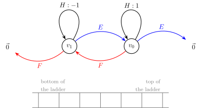
We can summarize these results in the following diagram.
The circles represent the basis vectors v_0, v_1.
Blue arrows: The action of applying the linear transformation \rho(E) on v_1 gives v_0, and applying \rho(E) on v_0 gives zero.
Red arrows: Similarly for \rho(F), it “brings” v_0 to v_1, and v_1 to zero.
Black arrows: the basis vectors v_0 and v_1 are the eigenvectors of \rho(H), with eigenvalues 1 and -1, respectively.
On the bottom of the image I put a ladder, with v_0 at its top and v_1 at its bottom. Right now it doesn’t make much sense to think of a ladder with only two rungs, but you can already think ahead and see where we’re going: representations in higher-dimensional spaces will give a ladder with more rungs, and the picture will become clearer.
Now, let’s move on to the next representation
13.22 the adjoint representation
In this representation, elements of the algebra are represented as linear operators (matrices) that operate on vectors in a 3d vector space. We need to define a basis for this space. In the 2d case of the standard representation, we chose the basis v_0=(1\,0)^T and v_1=(0\,1)^T. It would be natural to choose this time the basis
But that’s not what we will do. Instead, we already have a perfectly good basis to choose from, the three algebra elements E,H,F themselves!
This can feel truly weird and baffling. The elements E,H,F are at once:
The basis vectors of a 3d vector space.
The linear operators that operate on the basis vectors.
Actually, the second point is not quite precise. It’s not the elements E,H,F themselves that are the linear operators, but their adjoint representations: \rho_\text{adj}(E),\rho_\text{adj}(H),\rho_\text{adj}(F).
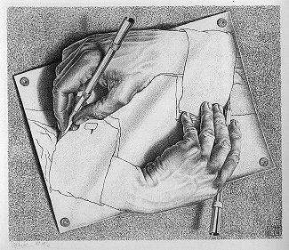
The special feature of the adjoint representation is that (representations of) elements in the algebra act on themselves. Choose your prefered metaphor here: a snake biting its own tail, a person lifting themselves by their bootstraps, or, my preferred, Escher’s Drawing Hands.
To determine the exact translation rule \rho_\text{adj}, that converts abstract algebra elements into 3\times3 matrices, we ask the question:
How should an algebra element X act on another algebra element Y?
Again, we perform the ultimate “reduce, reuse, recycle” act in the whole of Mathematics, and we use the special operation that makes \mathfrak{sl}(2) rise above being simply a vector space and become an algebra: the bracket. That is to say, how does (the representation of) X act on an element Y? Like this:
\rho_\text{adj}(X)Y = [X,Y]
Another common way to write the same thing is
\text{ad}_X(Y) = [X,Y].
This is the time to remember the Jacobi identity we saw before:
[X,[Y,Z]] +[Y,[Z,X]] + [Z,[X,Y]] = 0.
Just before we got to this nice form, we had it like this:
[X,[Y,Z]] = [[X,Y],Z] + [Y,[X,Z]],
which will prove useful now. By writing \text{ad}_X=[X,-] the act of “bracketing with X”, we can rewrite the Jacobi identity as
This is just like the product rule! The Jacobi identity says that “bracketing with X” distributes over a bracket exactly the way differentiation distributes over a product. That’s incredible! An operator with that property is called a derivation. So seen under a different light, the somewhat mysterious choice of reusing the bracket operation to define the adjoint representation is actually a very natural choice, because it is the only choice that makes \text{ad}_X a derivation.
Let’s find out now the precise expression of the 3\times3 matrices representing each of the elements E,H,F. For that, we need two things.
assume we want to know how the representations of the elements E,H,F act on a generic vector Y in this 3d space:
Y = aE + bH + cF.
On the right-hand side, we used E,H,F as basis vectors that span the 3d space, therefore Y is simply a linear combination of them. If we determine that the basis vectors are always ordered like E,H,F, we can express the vector Y as
Y = \begin{pmatrix}a\\b\\c\end{pmatrix}.
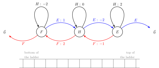
I’ll come back to the image of the ladder introduced in the standard representation. I want to know how each of the operators \text{ad}_E,\text{ad}_H,\text{ad}_F acts on each of the basis vectors E,H,F:
Of course, the this is exactly the same information as we obtained in the 3\times3 matrices we’ve just derived. Picture each outcome above as a column vector and you’ll understand why.
The ladder has three rungs now. Applying the operator E makes us go up the ladder, until we reach its top and fall into the abyss: \text{ad}_E(E)=0. The same goes for F, it brings us down the ladder, and when we step off the bottom rung we also fall into the abyss: \text{ad}_F(F)=0. Intuitively enough, the elements E and F are called step operators, or raising and lowering operators. The scalars that appear in the red and blue arrows are called ladder coefficients. The property that by applying these step operators enough times we will eventually get a zero has a name: nilpotent. Nil means zero or null, and potent means power, meaning that applying a power of these operators onto a basis vector yields zero. For example, start from the bottom rung F and apply E three times: E(E(E(F)))=E^3F=0. So E and F are nilpotent step operators.
The operator H has a few names, depending on the context. In mathematics it is known as the Cartan element, in Quantum Physics it is called the diagonal or measuring operator, and in focusing on the ladder analogy, it is called the level-counting or number operator. In any case, the operator H plays the role of a weight generator: we apply it to any basis element and we get back the same basis element multiplied by a weight. In other words, all basis elements E,H,F are eigenvectors of the operator H, with eigenvalues 2,0,-2, respectively.
13.23 irreducible representations
We have now seen three representations of \mathfrak{sl}(2): the 1D trivial representation, the 2D standard representation, and the 3D adjoint representation. These are not just isolated examples. They are the first three irreducible representations of \mathfrak{sl}(2). Irreducible means that the representation cannot be decomposed into smaller invariant pieces. In the ladder picture, this means the ladder is connected from bottom to top by the actions of E and F. If it were possible to decompose the representation into smaller subspaces, this would mean that the ladder would be split into 2 or more parts, not mutually accessible by applying the step operators.
To make sense of an n-dimensional irreducible representation, we look for a tool that helps us organize the n-dimensional space into neat, independent subspaces. The operator H is such a tool. To explain why, we need to talk about weights.
13.24 weights
Let’s write down the representation of H for the standard and the adjoint representations:
The diagonals of each matrix show precisely the eigenvalues of the basis vectors for the 2D and 3D representations. Take a look at the ladder diagrams from before, and notice the numbers assigned to the black loopy arrows.
By applying the operator H to a vector in an n-dimensional space, we are acting like a measuring device asking: “Hey vector, which rung of the ladder are you on?” To see how this works, let’s test it on an arbitrary vector v in our 3D vector space (the adjoint representation), where our basis vectors are the algebra elements themselves: (v_0, v_1, v_2) = (E, H, F). If we write v as a general linear combination v = aE + bH + cF, applying H yields:
While this output is not a simple scalar multiple of our input vector, look closely at the structure of the result: H did not scramble our ingredients. The E component remained strictly along the E direction (scaled by +2), the H component was scaled by 0, and the F component remained along the F direction (scaled by -2). Contrast this with the step operator E:
The ingredients bleed into one another, shifting across dimensions and destroying the original vector’s anatomy. The E direction now depends on the original direction in H (because of the coefficient b), and the H direction depends on the previous F direction (because of c). A similar thing happens to the step operator F, it also mixes the different directions.
This reveals the true power of H: it acts like a prism or frequency analyzer. Because its action is diagonalizable, H is the unique operator capable of reading a complex, multidimensional space and separating it into clean, independent components without tangling them together. When we feed H a pure basis state, it isolates its numerical tag (its weight) allowing us to construct the vertical scaffolding of our ladder:
If v = 1E + 0H + 0F, then \rho(H)E = \mathbf{+2}E \implies \text{weight is } +2
If v = 0E + 1H + 0F, then \rho(H)H = \mathbf{0}H \implies \text{weight is } 0
If v = 0E + 0H + 1F, then \rho(H)F = \mathbf{-2}F \implies \text{weight is } -2
Let’s construct an entire ladder from the top down. Let’s start at the very top rung, the highest weight vectorv_0, where E v_0 = 0. Once we are on the top rung, we just repeatedly apply the lowering operator F to build the entire n-dimensional ladder from scratch! Because F is nilpotent, this ladder is guaranteed to terminate. The same idea would work if we started from the base rung and climbed up the ladder with E. Each of these rungs represents an eigenvector of the representation of H, and its associated eigenvalue is the weight. The basis of the vector space for an n-dimensional representation is written as
V_\lambda =
\left\{
v \in V \mid Hv=\lambda v
\right\} =
\text{ weight space}
What is the relationship between weights in neighboring rungs? Take a given rung v with weight \lambda. What are the weights of the rung above it (Ev) and below it (Fv)?
\begin{align*}
H(Ev) &= HE\cdot v \\
&= \left( EH + \underbrace{[H,E]}_{HE-EH} \right)\cdot v \\
&= E(Hv) + 2Ev \\
& = \lambda E v + 2Ev \\
&= (\lambda+2)Ev
\end{align*}
We found that the weight of the rung above v is \lambda+2. A similar calculation works for the rung below v, namely Fv:
\begin{align*}
H(Fv) &= HF\cdot v \\
&= \left( FH + \underbrace{[H,F]}_{HF-FH} \right)\cdot v \\
&= F(Hv) - 2Fv \\
& = \lambda F v - 2Fv \\
&= (\lambda-2)Fv
\end{align*}
The weight of the rung below v is \lambda -2.
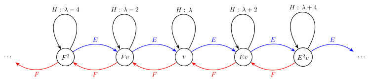
The diagram belows shows the general ladder structure, and the weights between neighboring rungs of the ladder.
13.25 ladder coefficients
Now that we know how the weights of neighboring rungs of the ladder relate to each other, the very last thing is to learn how the operations E and F morph a state into a higher or lower one.
Let’s assume an n-dimensional space, where v_0 is the highest rung of the ladder, that is, by stepping one more step up we “fall off it”: Ev_0=0. Likewise, v_{n-1} is the lowest rung, and stepping down from it also gives us zero: Fv_{n-1}=0. Finally, let’s call \lambda the weight of the highest rung v_0. That is to say:
Hv_0 = \lambda v_0
Hv_1 = (\lambda-2) v_1
Hv_2 = (\lambda-4) v_2
and in general Hv_k = (\lambda-2k) v_k
If we are at a general rung v_k, what do we get after stepping up once? That is to say, in the equation
Ev_k = c_k v_{k-1},
\tag{$\star$}
what is c_k? One value of this ladder coefficient is known already:
E v_0 = c_0 v_{-1}=0 \longrightarrow c_0=0.
We will find an recursion expression for c_k by starting with the following equation:
Let’s try to get a closed-form expression for c_k. Let’s compute the first ladder coefficients and see if we can identify a pattern there. To make my life a bit easier, I’ll shift the index k+1 to k in the recursion expression, so we have
c_k= c_{k-1}+\lambda-2(k-1).
k=0: \quad c_0 = 0
k=1: \quad c_1 = \lambda
k=2: \quad c_2 = 2(\lambda - 1)
k=3: \quad c_3 = 3(\lambda - 2)
k=4: \quad c_4 = 4(\lambda - 3)
k=5: \quad c_5 = 5(\lambda - 4)
In the first line, k=0, we did not use the recursion expression. We defined this as true because we are at the highest rung of the ladder, which means that applying E to v_0 has to give zero.
It’s pretty clear what the pattern is. A general ladder coefficient is
c_k = k(\lambda - k + 1).
Conclusion: this analysis shows us how the operator E converts a given basis vector v_k to v_{k-1}:
Ev_k = k(\lambda - k + 1) v_{k-1}
13.26 weight values
From the results above, we can not only determine that the weights of neighboring basis vectors differ by 2, but we can actually determine their values. Let’s see how.
Assume an irreducible representation of dimension n+1, whose basis vectors are:
V_\lambda: \text{ basis}=\{ v_0,v_1,\ldots,v_n \}
The operator F brings one basis vector to another down the ladder, until we fall off into the abyss:
Fv_k \propto v_{k+1},\qquad Fv_n=0.
The operator E brings one basis vector to another up the ladder, like this:
Ev_k = k(\lambda - k + 1) v_{k-1}.
To find the precise values of the weights, we start at the very bottom of the ladder. Applying F to v_n gives zero, meaning that:
Fv_n=0 \longrightarrow v_{n+1} = 0.
We also know that The operator E, applied to this zero vector v_{n+1} gives, according to the relationship we already found before,
E v_{n+1} = c_{n+1}v_n \longrightarrow E\cdot 0 = c_{n+1}v_n
But we know that v_n is not zero, so c_{n+1} must be:
Conclusion: the highest weight of an irreducible representation of dimension n+1 equals n. Going down each rung in the ladder decreases weights by 2, until we get to the bottom rung, whose weight must be
This has been a very long chapter, it’s time to wrap it up.
From first principles, we derived the \mathfrak{sl}(2) algebra, which is derived from the SL(2) group. We got to know its basis elements E,H,F and how they interact through the Lie bracket. We then developed concrete realizations of the algebra, when the basis elements are treated as linear operators that act on n-dimensional vector spaces. We did that for the trivial, standard and adjoint representations, and then we generalized the ladder picture for any finite-dimensional irreducible representation.
The next chapters will show the relevance of the \mathfrak{sl}(2) algebra in various important applications in Physics. Our hard work will pay off handsomely.