6  intractable bayesian inference

In the previous section, we solved a simple 2x2 grid where the mouse only had to worry about whether a fox was present or absent. While that was a great starting point, the real world is rarely that discrete. To move toward a more realistic model, we must consider the world as a continuous space.

6.1 moving to continuous states

Imagine that the mouse is no longer just asking “is there a fox?” but is instead trying to estimate the distance of the fox from the burrow.

• External state x^\star: The physical, objective distance of the fox (e.g., 100 meters).
• Hidden state x: The latent state in the mouse’s model, corresponding here to fox distance. The mouse does not observe x directly; it must infer a belief distribution over x from sensory data.
• Sensory outcome y: The continuous intensity of the fox’s scent reaching the mouse’s nose.

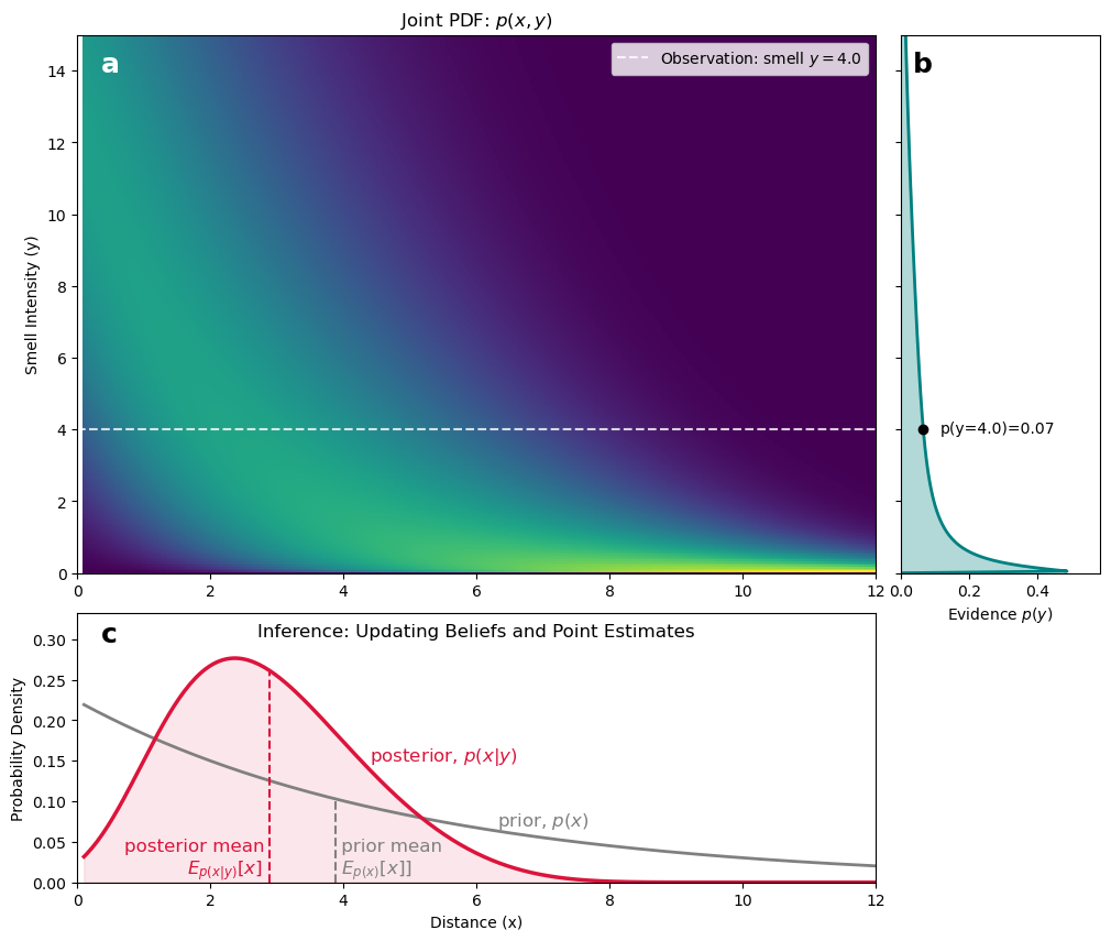
In this scenario, the mouse’s generative model is no longer a simple table. It is a continuous joint probability density function (PDF), p(x, y). This function maps how likely a specific smell intensity y is, given a specific distance x, weighted by how likely the mouse thinks that distance was in the first place (the prior).

import numpy as np
import matplotlib.pyplot as plt
from scipy.stats import gamma
from matplotlib.colors import PowerNorm

# 1. Setup the axes
x = np.linspace(0.1, 12, 300) 
y = np.linspace(0, 15, 300)   
X, Y = np.meshgrid(x, y)

dx = x[1] - x[0]
dy = y[1] - y[0]

# 2. Define the Generative Model
prior_pdf = np.exp(-0.2 * x)
prior_pdf /= np.sum(prior_pdf) * dx 

k = 1 + 5 * np.exp(-0.5 * x) 
mean_y = 15 * np.exp(-0.4 * x)
theta = mean_y / k
likelihood_pdf = gamma.pdf(Y, a=k, scale=theta)

# 3. Compute Joint PDF
joint_pdf = likelihood_pdf * prior_pdf[None, :]

# 4. Marginal Likelihood (Evidence)
evidence_y = np.sum(joint_pdf, axis=1) * dx

# 5. Inference for a specific observation (y=4.0)
obs_y_val = 4.0
y_idx = np.argmin(np.abs(y - obs_y_val))
numerator_slice = joint_pdf[y_idx, :]
evidence_scalar = evidence_y[y_idx]
posterior_pdf = numerator_slice / evidence_scalar
posterior_pdf /= np.sum(posterior_pdf) * dx

# 6. Calculate Centers of Mass (Expected Values)
# E[x] = sum(x * p(x)) / sum(p(x)) -- since they are normalized, the denominator is 1
com_prior = np.sum(x * prior_pdf) * dx
com_posterior = np.sum(x * posterior_pdf) * dx

# 7. Plotting
fig = plt.figure(figsize=(12, 10))
gs = fig.add_gridspec(2, 2, width_ratios=[4, 1], height_ratios=[4, 2], hspace=0.1, wspace=0.05)

# Top Left: Joint PDF
ax_main = fig.add_subplot(gs[0, 0])
im = ax_main.pcolormesh(X, Y, joint_pdf, shading='auto', cmap='viridis', norm=PowerNorm(gamma=0.3))
ax_main.axhline(obs_y_val, color='white', linestyle='--', alpha=0.8, label=f'Observation: smell $y={obs_y_val}$')
ax_main.set_ylabel('Smell Intensity (y)')
ax_main.set_title('Joint PDF: $p(x, y)$')
ax_main.legend()

# Top Right: Evidence Sidebar
ax_evid = fig.add_subplot(gs[0, 1], sharey=ax_main)
ax_evid.plot(evidence_y, y, color='teal', lw=2)
ax_evid.fill_betweenx(y, 0, evidence_y, color='teal', alpha=0.3)
ax_evid.set_xlabel('Evidence $p(y)$')
ax_evid.set(ylim=(0, 15),
            xlim=(0, evidence_y.max() * 1.2)
)
y4_idx = np.argmin(np.abs(y - 4.0))
ax_evid.plot(evidence_y[y4_idx], y[y4_idx], 'ko', label=f'Evidence at $y={obs_y_val}$')
ax_evid.text(evidence_y[y4_idx] + evidence_y.max()*0.1, y[y4_idx], f'p(y=4.0)={evidence_y[y4_idx]:.2f}', va='center', ha='left', fontsize=10)
plt.setp(ax_evid.get_yticklabels(), visible=False)

# Bottom: Prior vs Posterior with Centers of Mass
ax_inf = fig.add_subplot(gs[1, 0], sharex=ax_main)
ax_inf.plot(x, prior_pdf, color='gray', linestyle='-', lw=2, label='Prior $p(x)$')
ax_inf.plot(x, posterior_pdf, color='crimson', lw=2.5, label='Posterior $p(x|y)$')
ax_inf.fill_between(x, 0, posterior_pdf, color='crimson', alpha=0.1)

ax_inf.text(7, 0.07, r"prior, $p(x)$", color='gray', fontsize=12, ha='center')
ax_inf.text(5.5, 0.15, r"posterior, $p(x|y)$", color='crimson', fontsize=12, ha='center')
ax_inf.text(com_prior, 0.01, " prior mean\n" + r" $E_{p(x)}[x]]$", color='gray', fontsize=12, ha='left')
ax_inf.text(com_posterior, 0.01, "posterior mean \n" + r"$E_{p(x|y)}[x]$  ", color='crimson', fontsize=12, ha='right')
# Add Vertical Lines for Centers of Mass
x_com_prior_idx = np.argmin(np.abs(x - com_prior))
x_com_posterior_idx = np.argmin(np.abs(x - com_posterior))
ax_inf.plot([x[x_com_prior_idx]]*2, [0, prior_pdf[x_com_prior_idx]], '--', color='gray', label=f'Prior Mean: {com_prior:.2f}')
ax_inf.plot([x[x_com_posterior_idx]]*2, [0, posterior_pdf[x_com_posterior_idx]], '--', color='crimson', label=f'Posterior Mean: {com_posterior:.2f}')
# ax_inf.axvline(com_prior, color='gray', linestyle='--', alpha=0.6, label=f'Prior Mean: {com_prior:.2f}')
# ax_inf.axvline(com_posterior, color='crimson', linestyle='--', alpha=0.8, label=f'Posterior Mean: {com_posterior:.2f}')

ax_inf.set_xlabel('Distance (x)')
ax_inf.set_ylabel('Probability Density')
ax_inf.set_title('Inference: Updating Beliefs and Point Estimates', y=0.88)
ax_inf.set(xlim=(0, 12),
           ylim=(0, max(prior_pdf.max(), posterior_pdf.max()) * 1.2)
           )

ax_main.text(0.03, 0.97, r"a", transform=ax_main.transAxes,
         horizontalalignment='left', verticalalignment='top',
         fontweight="bold", color="white", fontsize=18)
ax_evid.text(0.06, 0.97, r"b", transform=ax_evid.transAxes,
         horizontalalignment='left', verticalalignment='top',
         fontweight="bold", color="black", fontsize=18)
ax_inf.text(0.03, 0.97, r"c", transform=ax_inf.transAxes,
         horizontalalignment='left', verticalalignment='top',
         fontweight="bold", color="black", fontsize=18)

plt.show()

Assume that the mouse started with a prior probability density for the fox’s distance as shown by the gray curve in panel c. The expected value (center of mass) of this prior is 3.87 (in standard mouse units). The mouse then receives a sensory observation of y=4.0. The mouse uses its internal generative model to figure out what this means. The generative model is the joint PDF shown in panel a, which encodes the likelihood of observing different scent intensities at different distances, multiplied by the prior belief about those distances. By slicing through this joint PDF at the observed scent intensity of y=4.0 (gray dashed line), the mouse can find the numerator of Bayes’ rule, p(x, y=4.0). To get the posterior, the mouse needs to normalize this slice by the evidence p(y=4.0). The full curve for the evidence p(y) is shown in panel b, and it can be calculated by integrating the joint PDF over all distances x, that is, integrating over the horizontal axis of panel a. This integral gives us the marginal probability of observing that scent intensity, regardless of the distance. The value of the evidence at y=4.0 is shown as a black dot in panel b, and it equals 0.07. This value is the denominator in Bayes’ rule. Strictly speaking, this is not the probability of observing exactly y=4.0, but the probability density around that sensory value. Finally, the mouse divides the slice of the joint PDF at y=4.0 by this evidence value to get the posterior PDF over distances given the observed scent intensity. This is the red curve in panel c. The center of mass of the posterior is 2.89, which is closer than the prior mean of 3.87, indicating that after sniffing a smell intensity of 4.0, the mouse now thinks that the fox is likely closer than it previously thought.

Easy, right?

6.2 the problem of degeneracy

At first glance, this seems like a “simple enough” upgrade to the example from the previous section. If the mouse gets a smell intensity of y=4, it can just look at the corresponding “slice” of the joint PDF and find the most likely distance. In our Python “cartoon,” this is a trivial numerical task.

However, real-world sensory data is degenerate. This means that a single sensory input (a faint smell) could be caused by many different configurations of the world.

1. The fox is far away on a breezy day.
2. The fox is very close, but the wind is blowing the scent away from the burrow.
3. The fox is medium-distance, but the mouse has a stuffed nose (sensor noise).

If the mouse only models “distance”, its likelihood mapping p(y|x) must be extremely “blurry” to account for all that wind-related uncertainty. A model that collapses all this uncertainty into distance alone becomes very broad: the same smell intensity is compatible with many possible distances.

6.3 the problem of generalization

There is an even deeper problem. In the 2×2 example, it was reasonable to imagine that the mouse had learned the full likelihood matrix from experience. But in a continuous, high-dimensional world, this is impossible. The mouse has never experienced every possible combination of distance, wind direction, wind speed, humidity, vegetation, and fox behavior. Therefore, it cannot simply store a giant likelihood table.

To survive, the mouse needs a generative model with structure. It must assume that smells behave in lawful ways: they tend to weaken with distance, drift with wind, and become noisier under turbulent conditions. These assumptions allow the mouse to generalize beyond direct experience. In other words, the generative model is not just memory; it is a compressed, structured model of how hidden causes generate sensory data.

But even with structure, inference remains difficult. Once the model contains many hidden causes, the mouse must infer a whole configuration of the world, not just one variable. This brings us to the curse of dimensionality.

6.4 the curse of dimensionality

To gain precision, the mouse must expand its hidden state x into a high-dimensional vector. It must model not just distance, but also wind velocity, wind direction, and turbulence, not to speak of the fox’s behavior and the possibility that there are multiple foxes. These are “nuisance variables”—the mouse doesn’t care about the wind for its own sake, but it must infer the state of the wind to “de-noise” the smell of the fox.

As we add these necessary dimensions (distance, angle, velocity, wind speed, turbulence, humidity, etc.), our “easy” Bayesian solution falls apart:

1. The Integral Problem: To find the evidence p(y), the mouse must now integrate over all these dimensions simultaneously.

p(y) = \int \int \int \dots \int p(y|x_1, x_2, \dots, x_n) p(x_1, x_2, \dots, x_n) dx_1 dx_2 \dots dx_n

2. Computational Collapse: If we used the same 300-point grid from our Python script for 10 dimensions, we would need 300^{10} calculations. That is roughly 5 \times 10^{24} operations—far more than any biological brain can compute in the split second needed to escape a predator. If we tried to solve the posterior by explicitly evaluating the joint density on a grid, as we did in the simple Python example, the computation would explode.

6.5 the need for a shortcut

This is the statistical inverse problem in its true form. The sensory data are generated by hidden causes, but many different hidden causes can produce the same sensory outcome. Exact Bayesian inference tells us what the ideal posterior should be, but in high-dimensional environments computing it directly becomes impossible. Variational inference provides a shortcut: instead of calculating the exact posterior, the system maintains an approximate belief distribution q(x) and adjusts it to better explain the sensory data. This move—from exact inference to approximate inference—is the mathematical doorway into active inference.