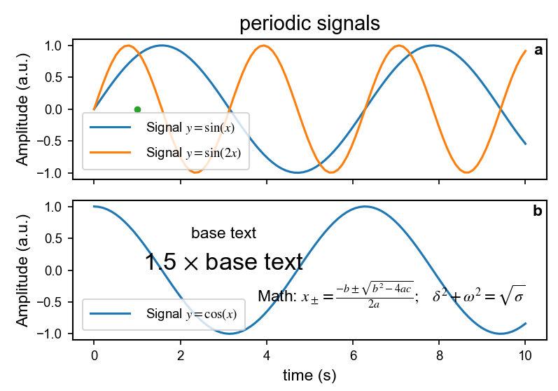
1  graph parameters

import libraries:

import matplotlib.pyplot as plt
import numpy as np

Download the file plot_style.py.

Explanation:

• width_fraction: default 1.0. Assume the generated image will be included in a latex document. If you want this image to occupy 90% of the width of the text, then you will write something like \includegraphics[width=0.9\textwidth]{my_figure.pdf}. In this case use width_fraction=0.9. If you don’t need any of this, just choose 1.0.
• view_scale: default 1.0. Often, the figure generated looks too small on a jupyter notebook, and it’s hard to know if everything is in the right place where we wanted. While developing the figure, you can make it look larger, e.g. making it twice as large by typing view_scale=2.0. Once you’re satisfied with the image, and you’re ready to produce the final pdf version, make it the intended size using view_scale=1.0.
• columns: default 1. Will this figure be embeded in a 1-column latex document, or a 2-column latex document?
• height_ratio: default 0.618. This is the height dimension relative to the width.

from plot_style import set_pub_style
style = set_pub_style(width_fraction=0.9, columns=1, view_scale=1.5, height_ratio=0.7)
# metadata = set_pub_style(width_fraction=0.9, columns=1, view_scale=2.0, height_ratio=0.7)

# this is needed to prevent the figure from being cropped when shown in a Jupyter notebook.
# what we see on the screen is the same as what we get in the saved PDF file.
%config InlineBackend.print_figure_kwargs = {"bbox_inches": None}

fig, ax = plt.subplots(2, 1, sharex=True)
fig.subplots_adjust(left=0.13, right=0.98, top=0.90, bottom=0.13, hspace=0.15, wspace=0.02,)

x = np.linspace(0, 10, 100)
ax[0].plot(x, np.sin(x), label=r"Signal $y = \sin(x)$")
ax[0].plot(x, np.sin(2*x), label=r"Signal $y = \sin(2x)$")
ax[1].plot(x, np.cos(x), label=r"Signal $y = \cos(x)$")

ax[0].plot([1], [0], marker="o")
ax[1].text(3, 0.5, r"base text", ha="center")
# use the `style` dictionary to modify a parameter.
ax[1].text(3, 0.0, r"1.5 $\times$ base text", ha="center", fontsize=1.5 * style["font"]["base"],)
ax[1].text(10, -0.5, r"Math: $x_\pm=\frac{-b\pm\sqrt{b^2-4ac}}{2a};\quad \delta^2+\omega^2=\sqrt{\sigma}$", ha="right")

ax[0].set_ylabel("Amplitude (a.u.)")
ax[0].legend()

ax[1].set_xlabel("time (s)")
ax[1].set_ylabel("Amplitude (a.u.)")
ax[1].legend(loc="lower left")

ax[0].text(0.99, 0.97, r"a", transform=ax[0].transAxes,
         horizontalalignment='right', verticalalignment='top',
         fontweight="bold")
ax[1].text(0.99, 0.97, r"b", transform=ax[1].transAxes,
         horizontalalignment='right', verticalalignment='top',
         fontweight="bold")

ax[0].set(title="periodic signals")
# fig.suptitle("periodic signals")

fig.savefig(
    "stam_graph.pdf",
    format="pdf",
    metadata=style["metadata"],
    bbox_inches=None,
)
fig.savefig(
    "stam_graph.png",
    format="png",
    bbox_inches=None,
)