Least Squares

How to fit a nonlinear function to data

Introduction

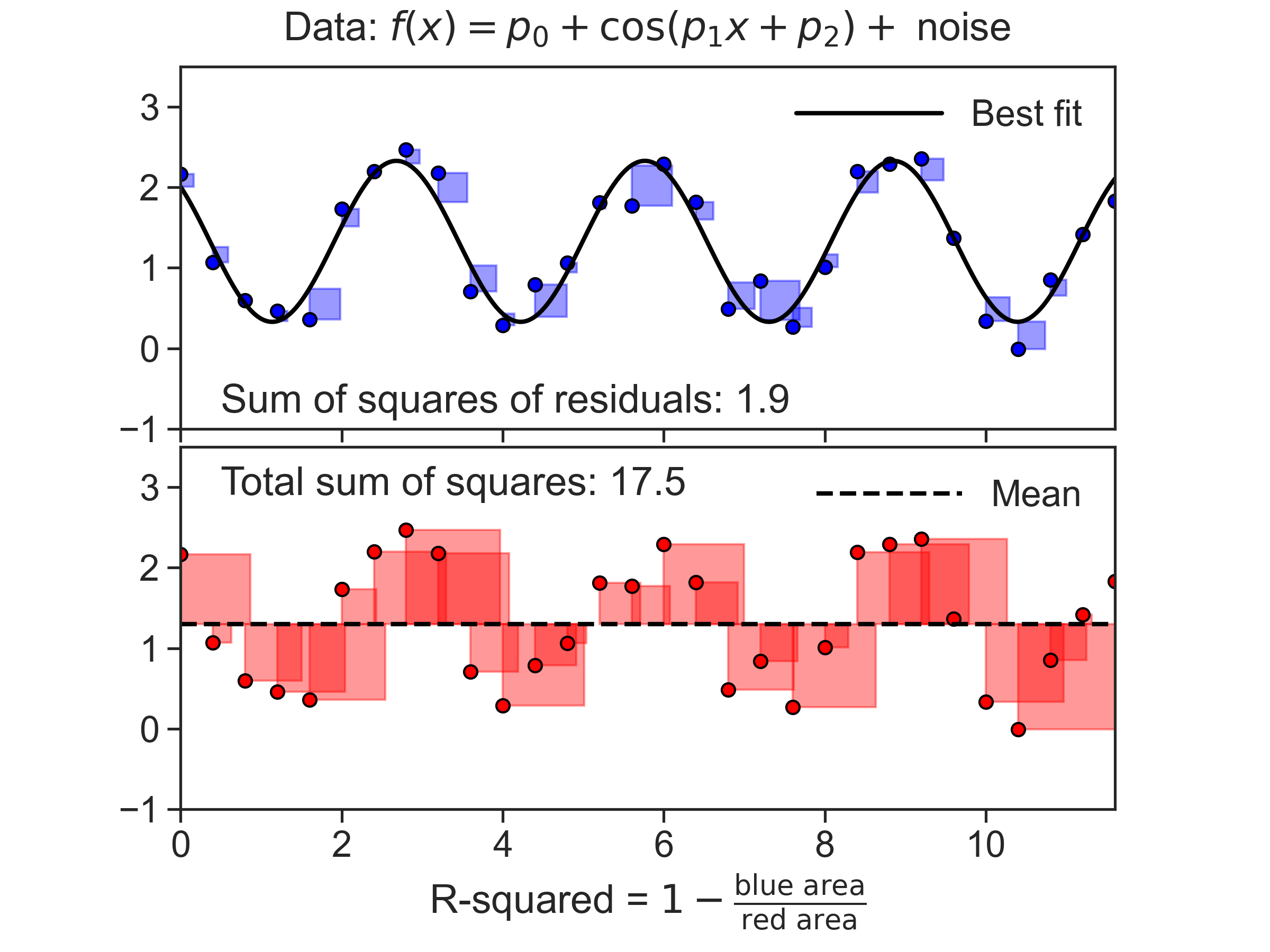
This code produces the figure above. It’s main tool is the curve_fit method, that allows us to fit any function to data, and get optimal parameter values.

The code

import matplotlib.pyplot as plt
import numpy as np
import matplotlib.gridspec as gridspec
import scipy.special
from scipy.optimize import curve_fit
import matplotlib.patches as patches
import seaborn as sns
sns.set(style="ticks", font_scale=1.5)

Define some functions

x = np.arange(0, 12, 0.4)

def func(x, par0, par1, par2):
    return par0 + np.cos(par1 * x + par2)


def add_rec(ax, c, v, col):
    ax.add_patch(
        patches.Rectangle(
            c,          # (x,y)
            np.abs(v),  # width
            v,          # height
            alpha=0.4,
            color=col
        )
    )

Now let’s plot some stuff

%matplotlib notebook

fig, [ax1, ax2] = plt.subplots(2, 1, figsize=(8,6), sharex=True, sharey=True,
                               subplot_kw={'aspect':'equal'}
                              )
fig.subplots_adjust(left=0.04, right=0.98, top=0.93, bottom=0.15,
                    hspace=0.05, wspace=0.02)
params = {#'backend': 'ps',
          'font.family': 'serif',
          'font.serif': ['Computer Modern Roman'],
          'ps.usedistiller': 'xpdf',
          'text.usetex': True,
          # include here any neede package for latex
          'text.latex.preamble': [r'\usepackage{amsmath}'],
          }
# the parameter values
par = (1.3, 2, 1)
# generating data with noise
y = func(x, *par) + (np.random.random(len(x)) - 0.5)
ax1.plot(x, y, marker='o', ls='None', markerfacecolor="blue", markeredgecolor="black")
ax2.plot(x, y, marker='o', ls='None', markerfacecolor="red", markeredgecolor="black")

# best fit
popt, pcov = curve_fit(func, x, y, p0=(1.5, 1.5, 2.5))  # p0 = initial guess
p0, p1, p2 = popt
# The total sum of squares (proportional to the variance of the data)
SStot = ((y - y.mean()) ** 2).sum()
# The sum of squares of residuals
SSres = ((y - func(x, p0, p1, p2)) ** 2).sum()
Rsquared = 1 - SSres / SStot
# plot best fit
h = np.linspace(x.min(), x.max(), 1001)
fit, = ax1.plot(h, func(h, p0, p1, p2), color='black', linewidth=2)
ax1.legend([fit], ["Best fit"], loc="upper right",
           frameon=False, handlelength=4)
# plot mean
mean, = ax2.plot(h, h * 0 + np.mean(y), ls='--', color='black', linewidth=2)
ax2.legend([mean], ["Mean"], loc="upper right", frameon=False, handlelength=4)

# plot blue and red squares
for ind in np.arange(len(x)):
    x0 = x[ind]
    y0 = y[ind]
    # print(x0,y0)
    v1 = y0 - func(x0, p0, p1, p2)
    v2 = y0 - y.mean()
    add_rec(ax1, (x0, y0), -v1, "blue")
    add_rec(ax2, (x0, y0), -v2, "red")

ax2.text(0.5, 2.9, r"Total sum of squares: {:.1f}".format(SStot))
ax1.text(0.5, -0.8, r"Sum of squares of residuals: {:.1f}".format(SSres))
# ax2.set_xlabel(
#          r"R-squared = $1 - \frac{\text{blue area}}{\text{red area}}$ = " +
#          "{:.2f}".format(Rsquared))
ax2.set_xlabel(
              r"R-squared = $1 - \frac{\mathrm{blue\ area}}{\mathrm{red\ area}}$"
              )
ax1.set_xlabel(
               r"Data: $f(x) = p_0 + \cos(p_1 x + p_2)+ $ noise ",
               labelpad=12
               )
ax1.xaxis.set_label_position("top")

ax1.set(xlim=[x.min(), x.max()],
        ylim=[-1, 3.5],
        xticklabels=[],
        yticks=np.arange(-1, 4)
       )
ax2.set(
        xticklabels=np.arange(0,13,2)
       )

fig.savefig("least-squares.png", dpi=300)

/Users/yairmau/opt/anaconda3/lib/python3.7/site-packages/ipykernel_launcher.py:70: UserWarning: FixedFormatter should only be used together with FixedLocator