Mechanisms behind facilitation–competition transition along rainfall gradients
- authors:
- Oded Hollander { }^{a,b} https://orcid.org/0009-0009-0484-2962
- Yair Mau { }^{b} https://orcid.org/0000-0001-6987-7597
- Niv DeMalach { }^{a} https://orcid.org/0000-0002-4509-5387
[b] Department of Soil and Water Sciences, Institute of Environmental Sciences, Robert H. Smith Faculty of Agriculture, Food and Environment, The Hebrew University of Jerusalem, Rehovot 76100001, Israel - Proceedings of the National Academy of Sciences, 2026
- Correspondence: Yair Mau (yair.mau@mail.huji.ac.il), Niv DeMalach (niv.demalach@mail.huji.ac.il)
- Received: May 29, 2026; | Accepted: July 16, 2026
- Keywords: Stress Gradient Hypothesis | aridity gradient | precipitation | plant–plant interactions | consumer–resource model
- doi: https://doi.org/10.1073/pnas.2615937123
- This article contains supporting information online at https://doi.org/10.1073/pnas.2615937123#supplementary-materials.
- How to cite:
O. Hollander, Y. Mau, & N. DeMalach, Mechanisms behind facilitation–competition transition along rainfall gradients, Proc. Natl. Acad. Sci. U.S.A. 123 (35) e2615937123, https://doi.org/10.1073/pnas.2615937123 (2026).
Edited by David Tilman, University of Minnesota College of Biological Sciences, St. Paul, MN; received May 29, 2026; accepted July 16, 2026
Significance
Shifts in woody cover, such as shrub encroachment and afforestation, are transforming drylands across the globe and directly impacting the herbaceous plants that provide critical forage. However, predicting whether woody plants will facilitate herb growth or inhibit it, and how these interactions change with rainfall, remains a major challenge. Our study translates the classic Stress Gradient Hypothesis into a quantitative, mechanistic model that includes both canopy shading and water dynamics. By unpacking these physical mechanisms, the framework explains why field studies often reach conflicting conclusions. More importantly, it provides a predictive tool to determine how changes in woody cover affect productivity, offering a transparent basis for planning conservation, restoration, and ecosystem management in water-limited environments.
Abstract
Woody cover is rapidly changing due to mortality, shrub encroachment, and afforestation, reshaping herbaceous communities and ecosystem functioning worldwide. Trees and shrubs often facilitate herb growth in dry sites but suppress it in wetter environments. Explanations for this facilitation-to-competition transition lack a clear link to resource competition theory, despite being a fundamental aspect of the broader Stress Gradient Hypothesis. While recent quantitative frameworks exist, explanations remain contested and have yet to reproduce the shift along a rainfall gradient from first principles. Here, we present a mechanistic framework consisting of two submodels: i) canopy shading, which reduces photosynthesis (competition) and evapotranspiration (facilitation), and ii) root effects, including water uptake (competition) and increased moisture via hydraulic redistribution (facilitation). We elucidate the conditions under which interactions shift from facilitation to competition. The models reproduce this reversal only when water is not the sole limiting factor at high rainfall or when woody density increases with precipitation. The two pathways leave distinct signatures: Canopy shading produces a hump-shaped pattern with maximum facilitation at intermediate stress, while the root pathway predicts a shift from positive to negative interactions as water availability increases. More generally, the reversal is robust across mechanisms and gradients: Enhanced infiltration can replace hydraulic redistribution, evaporative demand can replace rainfall, and combined canopy–root interactions preserve the transition. By translating a classic idea into a quantitative framework, this model enhances ecosystem management in a changing world.
Introduction
Global climate and land-use changes are rapidly reshaping woody vegetation worldwide (1, 2). These shifts are especially common in drylands, which cover about 40% of Earth’s land surface (3, 4). Many water-limited systems are losing woody cover due to widespread drought and fire (5). Conversely, other dry regions show woody expansion, driven by shrub encroachment (2, 6) and large-scale afforestation aimed at climate mitigation (1, 7). In these ecosystems, woody plants (hereafter, trees) strongly shape microclimate and resource availability, thereby influencing the abundance and distribution of herbaceous plants (hereafter, herbs) that sustain forage production and biodiversity in drylands (2, 6).
Trees are ecosystem engineers, altering the environment beyond simply consuming light and water (8). They can facilitate herb growth through canopy and root mechanisms. The canopy suppresses light availability, which reduces carbon assimilation (photosynthesis) but also lowers evapotranspiration and therefore water loss (9). This reduction in evapotranspiration also results from microclimatic buffering: slower wind speeds, higher humidity, and lower temperatures beneath the canopy (10). Tree roots not only extract water, thereby drying the soil, but can also increase soil moisture by enhancing infiltration (11) and potentially redistributing water from deeper to shallower soil layers through hydraulic lift (12, 13).
Rainfall amount often mediates the balance between these positive and negative effects. Meta-analyses find that trees typically benefit herbs at low rainfall but hinder them as rainfall increases (14–16). Even so, some studies report inconsistent neighbor effects along similar gradients (17), pointing to hidden thresholds or additional factors that alter the expected pattern.
Over the past three decades, the transition from facilitation to competition has largely been investigated through the lens of the Stress Gradient Hypothesis (SGH). This conceptual framework was proposed to explain why facilitation dominates under high abiotic stress (low rainfall), whereas competition prevails under benign conditions (18–23). The original explanations emphasized plant responses along water-stress gradients (20), but the hypothesis has since been applied to many other stress types (24, 25). The primary argument is that tree-mediated relief of water stress dominates under low rainfall, whereas shading-induced inhibition dominates under low stress (high rainfall) (9). These verbal arguments were later extended using phenomenological models that embedded spatial–temporal dynamics (26) and biodiversity feedbacks (27).
Despite its prominence, the SGH has been questioned both mechanistically and in terms of predicted patterns (9, 28–31). Some studies argue that species interactions become more strongly negative with rainfall (14), whereas others report a unimodal (hump-shaped) pattern in which facilitation peaks at intermediate stress and weakens under both severe aridity and benign conditions (29). This unimodal relationship is hypothesized to reflect a shifting balance between simultaneous, opposing processes: While trees facilitate herbs via canopy shading at intermediate stress, they outcompete them under benign conditions and ultimately suppress them under extreme aridity because belowground competition for scarce water overwhelms aboveground benefits. Resolving these discrepancies calls for quantitative models that explicitly represent resource dynamics and make assumptions transparent, allowing specific processes such as shading or water uptake to be identified as drivers that generate, sustain, or limit facilitation along the gradient.
Consumer–resource theory is the leading modeling framework for mechanistic explanations of species interactions (32–35). Yet, it has only recently been applied to the SGH (36, 37). These recent applications yielded insights into the role of trees in elevating resource availability during early succession (36) and into the joint effects of drought and grazing (37). However, they focused exclusively on root mechanisms and did not consider canopy shading, the main mechanism emphasized in the classical conceptual hypothesis (20). Crucially, and contrary to the SGH’s prediction of a facilitation-to-competition shift, these consumer–resource models produced an interaction sign that remained constant (either positive or negative) along the rainfall gradient, rather than a transition from facilitation to competition.
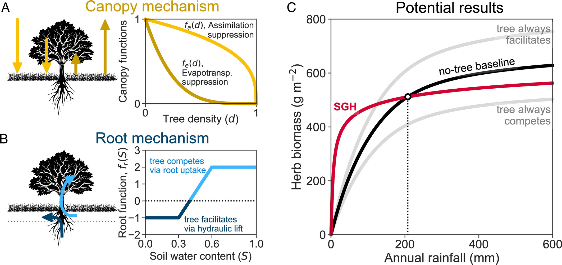
Here, we develop a minimal consumer–resource framework that generates the classic shift from facilitation to competition as rainfall (resource supply rate) increases. First, in the canopy submodel (Fig. 1A), trees suppress both carbon assimilation and evapotranspiration, but reduce evapotranspiration more strongly, a condition that enables net facilitation under water-limited conditions. Next, in the root submodel (Fig. 1B), trees simultaneously extract soil water (competition) and redistribute it upward from deep layers via hydraulic lift (facilitation), with the balance shifting as soil moisture increases. We show that both mechanisms can reproduce the SGH crossover (Fig. 1C): facilitation at low rainfall giving way to competition as rainfall rises. Furthermore, the transition is also preserved in combined models where canopy shading acts together with root water uptake, even without hydraulic lift, and can also arise when trees enhance infiltration.
Results
We developed a consumer–resource model that describes the coupled dynamics of herbs’ biomass and soil moisture as follows:
\begin{align*} \textbf{herb biomass:}&&\frac{dB}{dt} &= \overbrace{a\, {f_a}(d)\, {f_k}(B)B\, S}^{\text{growth}} - \overbrace{m\, B}^{\text{mortality}} \tag{1a} \\ \textbf{soil water:}&& \underbrace{n z_r}_{\mathclap{\substack{\text{active}\\ \text{soil depth} }}} \frac{dS}{dt} &= \underbrace{p}_{\text{precipitation}} - \underbrace{q_{s} S^c}_{\text{drainage}} - \underbrace{e_0\, {f_e}(d) B\, S}_{\text{evapotranspiration}} - \underbrace{{f_r}(S ,d)}_{\text{tree root}}. \\ &\tag{1b} \end{align*}
The first equation tracks the change in herb biomass (B) over time, which is governed by growth and mortality processes. The second equation represents the dynamics of soil moisture (S), which is influenced by gains from precipitation (p) and losses due to drainage, evapotranspiration, and a tree-root effect. Due to their much slower dynamics, trees are represented as a constant parameter for tree density (d representing canopy cover or root density). This parameter affects both the canopy-suppression factors on herb growth (f_{a}{(d)}) and on evapotranspiration (f_{e}{(d)}), as depicted in Fig. 1A. In the main model, tree density d is fixed to isolate the immediate resource-mediated mechanisms. We relax this assumption in SI Appendix, section S1, by considering precipitation-dependent woody cover. The impact of the root mechanism f_{r}{(S,d)} on soil water is depicted in Fig. 1B. We further assumed that when water and light are ample, other factors such as nutrients, pathogens or self-shading, limit herb growth, represented by a carrying capacity term f_{k}{(B)} = 1 - B/k. For simplicity, we started by investigating each mechanism sepa rately: When examining canopy effects, we removed root effects, and vice versa and only later tested the combined effects.
When water is the main limiting factor and tree density is constant, our model, like previous mechanistic models (36, 37), shows that the interaction between trees and herbs remains either facilitative or competitive along the entire precipitation gradient. However, a key finding is that the facilitation-to-competition transition does not arise from water limitation alone. Under constant tree density, an additional growth-limiting factor (represented by f_{k}{(B)}) is a necessary condition for the transition to occur (SI Appendix, section S2). When this condition is met, both the canopy and root mechanisms can produce a clear shift from facilitation to competition as precipitation increases. The following explores how each of these mechanisms drives this transition in steady-state solutions. An extended discussion on transient solutions can be found in SI Appendix, section S3.
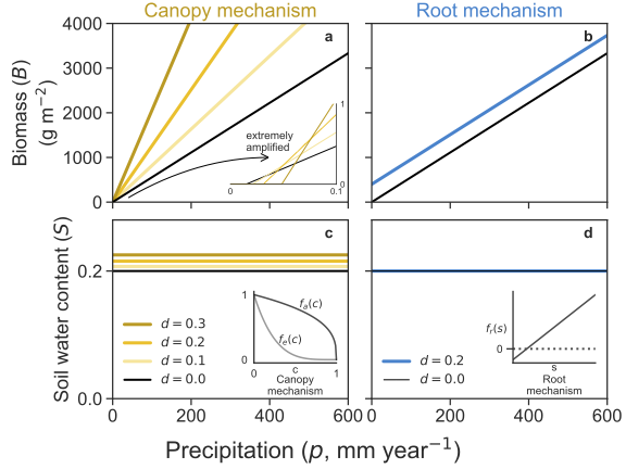
In the canopy mechanism, in the absence of trees, herb biomass increases with precipitation, showing a saturation pattern as the curve’s slope decreases (black line in Fig. 2A). With some trees (light curve), herb biomass is higher than the no-tree baseline at low precipitation but is reduced at higher precipitation levels, showing a clear transition from facilitation to competition. At very high tree density (dark curve), herb biomass is suppressed across the entire precipitation gradient.
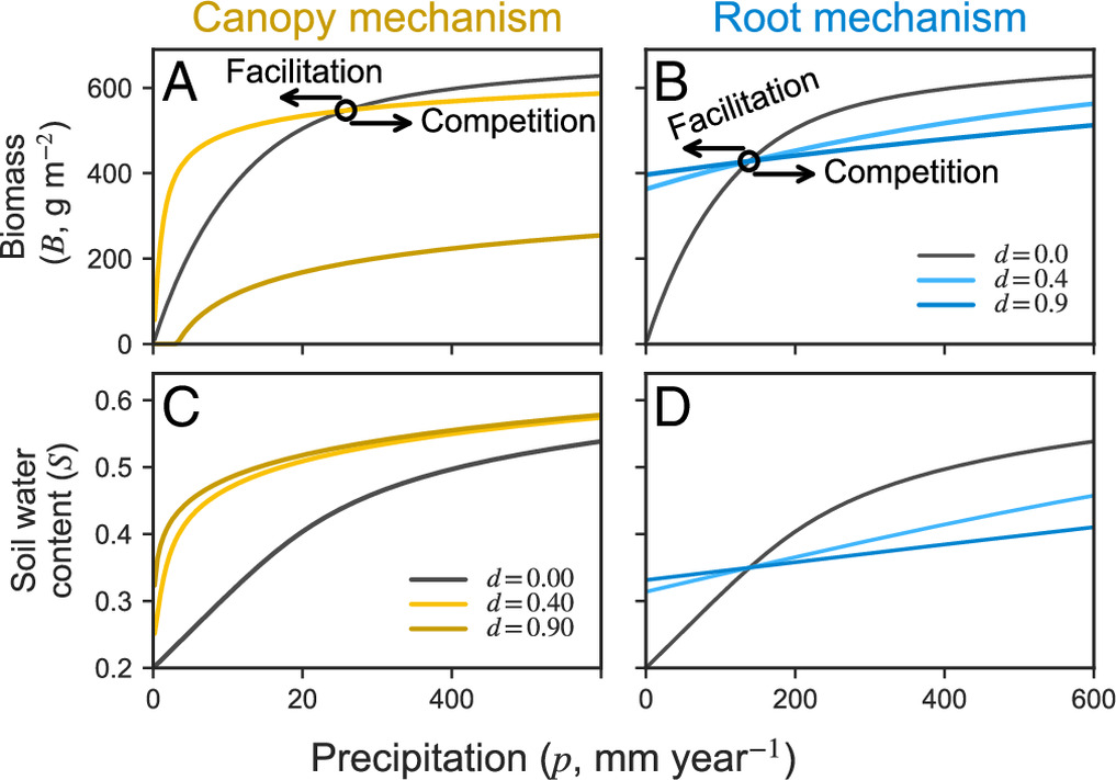
This pattern is a result of a tug of war between two opposing forces exerted by the trees. First, trees facilitate growth by providing shade, which reduces evapotranspiration and conserves soil water. This effect is represented by the function f_{e}{(d)}, leading to greater soil water availability relative to a no-tree environment (Fig. 2C). Second, trees inhibit herb growth by reducing light availability through the function f_{a}{(d)}. This factor, along with other limiting elements (captured by the carrying capacity term, f_{k}{(B)}), down-regulates herb assimilation. The combined effect is represented by the product f_{a}{(d)}f_{k}{(B)}.
At low precipitation, herb biomass is low, so the carrying capacity term f_{k}{(B)} is very weak (close to 1). In this dry scenario, the tug of war is mainly between the water-saving benefit of f_{e}{(d)} and the assimilation reduction effect of f_{a}{(d)}. When tree density is low, the extra soil water overpowers the minor loss in assimilation, facilitating herb growth (light curve in Fig. 2A). However, when tree cover is high, the reduction in assimilation becomes too strong, suppressing the herbs (dark curve). As precipitation increases, herb biomass also rises. This strengthens the carrying capacity term f_{k}{(B)} (making it closer to zero) and tips the balance. The combined competitive effect of reduced assimilation and carrying capacity (f_{a}{(d)}f_{k}{(B)}) becomes stronger than the facilitative effect of water conservation. In other words, under high rainfall, water is no longer the limiting factor, and therefore, the benefit of reduced water loss is not enough to compensate for the reduction in photosynthesis, leading to a transition from net facilitation to net competition.
For the root mechanism, all nonzero tree densities show a similar transition pattern: Herb biomass is higher than the baseline at low precipitation and lower at high precipitation (Fig. 2B). As tree density increases, both effects intensify along the precipitation gradient. This is because the tug of war between facilitation and competition is expressed by a single function, f_{r}{(S,d)}, which represents the net effect of tree roots on soil water available in the herb root zone.
This function captures the tipping of the balance as soil water content changes. At low soil water levels, tree roots can lift water from deeper soil layers to the herb root zone, facilitating growth. As soil water content increases, hydraulic lift is no longer possible. Beyond this point, roots begin to compete with herbs by taking up water from the same soil layer. Counterintuitively, the root term f_{r}{(S,d)} by itself does not produce a facilitation-to-competition switch (SI Appendix, section S2). With water as the only limiting resource (i.e., f_{k}{(B)} = 1), the equilibrium soil moisture S^{\star} is set by the consumer and is independent of the precipitation supply p [R* logic (33)]. Because f_{r} acts through S rather than directly through p, the sign of the interaction is fixed by whether S^{\star} lies below or above the hydraulic switching range, so it does not change along the rainfall gradient. However, when a second growth constraint is introduced through the carrying-capacity term f_{k}{(B)}, the outcome changes: As p increases, biomass approaches its limit and cannot deplete water further, so S^{\star} rises. This upward shift in S^{\star} carries the system across the hydraulic threshold, turning facilitative lift into competitive uptake and yielding the observed transition. Put simply, f_{k}{(B)} caps biomass at high rainfall, weakening consumption and allowing soil water to accumulate, which moves S^{\star} into the competitive domain of f_{r}{(S,d)}.
Notably, the two mechanisms produce very different biomass responses at low precipitation. In the canopy mechanism, precipitation is the only water source, so all curves must start from the origin, zero biomass at zero rainfall. A small initial increase in precipitation leads to stronger facilitation, which is visible as a widening gap between the low-tree-density curve and the no-tree baseline (light and black curves in Fig. 2A, respectively). This facilitative gap eventually narrows before disappearing at the transition to competition. In contrast, the root mechanism includes an additional water source: hydraulic lift from deeper soil layers during dry surface conditions. This allows herb biomass to persist even without precipitation. The gap between tree-density curves and the baseline shrinks steadily as precipitation increases, until it reaches the transition point. This distinct pattern in the biomass gap is key to understanding the contrasting responses in interaction intensity between the two mechanisms.
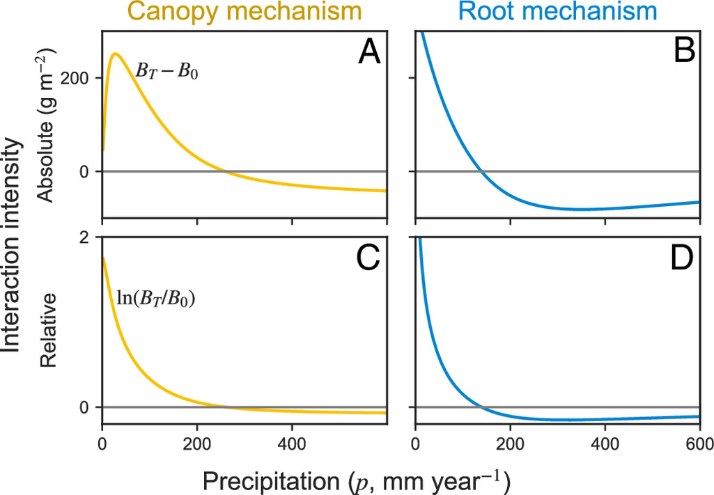
For the canopy mechanism, the interaction intensity based on the absolute difference is unimodal (Fig. 3A). This pattern directly results from the widening and eventual vanishing of the gap between the biomass curve with trees and the no-tree baseline curve, as previously discussed. However, when using the relative log response ratio (Fig. 3C), the interaction intensity decreases monotonically for p below the transition threshold. In contrast, the root mechanism yields monotonically decreasing positive interaction intensities, regardless of whether absolute difference or relative log response ratio is used. A broader discussion of the canopy mechanism’s interaction intensity in the full (p,d) parameter space is given in SI Appendix, section S4.
Discussion
The Stress Gradient Hypothesis has guided decades of work but has largely been articulated in verbal or phenomenological terms (9, 19, 20, 26, 27, 29, 30). We show that a minimal consumer–resource model linking canopy shading or root water redistribution to herb biomass generates the observed shift from facilitation to competition along rainfall gradients. Our model also specifies when the shift should and should not arise. Finally, the framework also clarifies the expectation on interaction intensity, with a mid-gradient peak in the facilitation under shading and a monotonic decline from positive to negative effect under the root pathway.
Our aim is to provide general insight and testable predictions rather than site-specific accurate description. Accordingly, the model is intentionally simple yet mechanistic: Water balance is explicit, and interaction signs emerge from the equations rather than being imposed a priori. This simplicity enables a thorough understanding of each parameter (SI Appendix, section S5).
This parsimony rests on two modeling choices that define the scope of the framework. First, the herbaceous layer is represented as a single biomass compartment governed by logistic growth. This formulation is most appropriate when herb biomass is dominated by a single species, but can also serve as an effective description of multispecies communities when species are similar in their growth and interaction parameters (SI Appendix, section S6). When communities contain strong trait differences among herbs, or when woody plants alter competitive interactions within the herbaceous layer, biomass responses may depend on community composition. In such cases, the model should be interpreted as a baseline against which composition-dependent responses can be compared.
Second, the deterministic rainfall–biomass curve should be interpreted as a mean-field expectation under constant environmental conditions. Its declining slope captures the general presumption that marginal biomass gains decrease as water limitation weakens (38, 39), but not the exact curvature or threshold of any particular site. Reproducing the scatter observed in natural systems would require extensions that incorporate spatial heterogeneity (e.g. soil) and time-varying drivers such as stochastic rainfall and grazing, producing a distribution of biomass outcomes rather than a single predicted value.
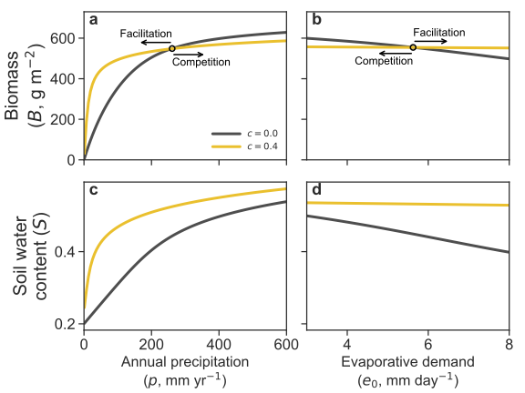
The framework also clarifies which stress gradients it add resses. The Stress Gradient Hypothesis has been invoked for many stress types (9, 18–23). Yet, as Maestre et al. noted, “Stress is not a precise concept, and therefore it is difficult to apply quantitatively to communities or ecosystems” (29). Here we focus on mechanisms tied directly to plant water balance, while recognizing that other stressors, such as freezing, toxicity, or salinity, and other interaction pathways, such as grazing protection, enhanced nutrient supply, spatial patterning, and tree density dynamics, are likely to require different model structures (31, 36, 37, 40, 41). The same framework can also be applied to evaporative demand, another driver of aridity influenced by temperature and humidity. This driver can change the magnitude of facilitation and competition and shift the transition point along the gradient. Still, the model consistently predicts a shift from net facilitation to net competition as water limitation relaxes (SI Appendix, Fig. S6 and section S7).
Notably, our model resolves the empirical question whether stress should be represented by resource supply rate (precipitation) or by resource abundance (soil water content) (9, 36, 37, 42). It shows that precipitation or evaporative demand are the appropriate measures for quantifying water stress in such systems (SI Appendix, section S8). Soil water content, in contrast, is not an independent driver but an emergent outcome of interacting processes including precipitation, evapotranspiration, biotic uptake, and substrate properties (9, 36, 42). Treating soil water as externally fixed cuts off these mechanistic links and removes the causal connection between resource supply and species interactions. Only when stress is parameterized as a supply rate can the facilitation–competition interplay characteristic of the SGH be captured (9, 36, 37, 42).
Canopy Mechanism
Shading is a ubiquitous factor in plant growth and community dynamics (43–46). This mechanism is central in conceptual models that generate the transition from facilitation to competition (9, 20). Our findings indicate that shading can simultaneously enhance and constrain growth, with implications far beyond tree–herb interactions.
In the model, shading acts solely by reducing light, so any reduction in radiation, whether caused from trees, slope aspect, buildings, or solar panels, should generate similar responses. In dry conditions, shaded hillslopes, north-facing in the northern hemisphere and the reverse in the southern hemisphere, should be more productive than sun-exposed slopes. In wet conditions, the pattern should reverse. Variation with slope aspect is a long-standing observation in botany (47, 48).
The model highlights several conditions that have seldom been investigated in theoretical and empirical studies along gradients. First, a necessary condition for facilitation under shading is that the proportional reduction in evapotranspiration with increasing shade exceeds the proportional reduction in photosynthesis. This condition can hold for many plants because assimilation often saturates at high light, whereas transpiration may continue to increase when water is not limiting (49–51). However, there are clear exceptions, such as species that require high light and are sensitive to shade. We therefore suggest that empirical tests of the canopy mechanism begin by verifying this assumption. From the theoretical side, consumer–resource models have traditionally assumed a full coupling of evapotranspiration and assimilation represented by a constant conversion factor of resource uptake to biomass, that is, fixed water-use efficiency (52, 53). While some degree of coupling is clearly expected, since both processes are shaped by stomatal conductance, assuming a fixed proportionality is unlikely to be realistic. We therefore relaxed this assumption, which was necessary for producing the SGH pattern.
For the transition from facilitation to competition to occur without a change in tree cover, another condition must be met. Under high rainfall, water must cease to be the main limiting factor (the carrying capacity effect). This implies that a qualitative switch is less likely when moving from an arid to a semiarid system if both remain water-limited. Instead, a switch is expected only when crossing into a system limited by another resource, such as nutrients (SI Appendix, section S9 which shows that carrying capacity is equivalent to an additional essential resource). This result may explain empirical studies that do not observe a shift along precipitation gradients (17, 29, 54, 55) and underscores that the transition should not be viewed as inevitable.
Alternatively, shading can lead to a facilitation-to-competition transition without introducing carrying capacity, but only when tree density increases with rainfall (SI Appendix, section S1). This occurs because at high tree cover, light becomes the primary limiting factor and offsets the positive effects of shading on water balance. This density effect can be further enhanced by photoinhibition, where moderate shade inhibits photosynthesis. We therefore recommend that future empirical studies quantify how tree density changes along the gradient and manipulate tree cover directly, or mimic shading with shade cloth. Such an approach is necessary to determine whether interaction outcomes change under a constant shade level (Fig. 2), or arise from shifts in canopy density along the gradient (SI Appendix, section S1).
To analyze the canopy mechanism, we adopted a two-layer simplification (56), assuming that because tree roots extend deeper than those of herbs, trees do not compete with herbs for the same soil water pool. This allowed us to isolate the consequences of reduced radiation. In most systems, some degree of rooting overlap is likely, so trees also consume water potentially available to herbs. Incorporating tree water uptake together with shading preserved the facilitation-to-competition transition, but shifts it to lower precipitation levels (SI Appendix, section S10).
Root Mechanisms
Below-ground, trees can modify herb water availability through several mechanisms, including competitive water uptake, hydraulic redistribution, and changes to soil infiltration properties. Root-mediated effects in natural settings can be highly variable because they depend on root architecture and soil properties (11, 57).
Under the hydraulic-lift mechanism, trees increase soil moisture under dry conditions and reduce it under wet conditions, so a transition from facilitation to competition can occur. Although we initially expected this transition to arise inevitably from this mechanism, we found that it occurs only when another factor limits biomass at high rainfall; otherwise, equilibrium soil moisture remains constant along the gradient.
Hydraulic redistribution has been documented across a wide range of ecosystems, including temperate forests (58), Mediterranean shrublands (59), and pine woodlands (60, 61), as well as semiarid savannas (62, 63). Yet in semiarid savannas, overstory trees were found to use nearly all hydraulically lifted water to meet their own transpirational demands, yielding net competition rather than facilitation for understory grasses (62). Moreover, the direction and magnitude of hydraulic redistribution can reverse between seasons and years even at a single site (63). We therefore treat hydraulic lift as a secondary and more uncertain mechanism relative to canopy shading. When combined with canopy shading (SI Appendix, section S10), a facilitation-to-competition transition still occurred, but we found no synergistic effect leading to a qualitatively new pattern. Instead, the combined response was intermediate between the patterns produced by each mechanism alone, with a subadditive effect such that the joint impact was weaker than expected from their separate effects. Alternatively, a more common way trees may increase soil moisture is by enhancing infiltration (11). While infiltration alone does not cause a facilitation-to-competition transition (37), our model shows that it can do so when combined with shading: Under low precipitation, the positive effects of increased infiltration dominate, whereas at high rainfall, the negative effects of shading prevail (SI Appendix, section S11).
Concluding Remarks
Our findings help reconcile conflicting reports on interaction strength along rainfall gradients by showing that the expected pattern depends first on the mechanism. Under the canopy pathway, the absolute difference in biomass is hump-shaped, with maximum facilitation at intermediate rainfall, whereas under the root mechanism, the interaction declines monotonically from positive to negative. A second source of variation is the metric, and this sensitivity applies to shading in particular: Only the absolute measure yields a unimodal pattern, whereas relative measures decline with rainfall, consistent with earlier suggestions (9).
Importantly, tree density further modulates these patterns of interactions along aridity gradients (SI Appendix, section S4). Hence, empirical patterns can only be interpreted accurately when tree density is quantified. Under low precipitation, facilitation peaks at intermediate density, while low and high tree densities weaken it. As precipitation increases, progressively lower densities are sufficient to shift the balance from facilitation to competition. Eventually, at high rainfall, even near-zero tree density reduces herb performance, so further changes in density no longer cause a qualitative shift (9).
Many empirical studies report a shift from facilitation to competition (14–16), and many do not (9, 28–31). In the lens of our framework, cases without a shift arise when i) other pathways dominate, for example, protection from herbivory, or ii) when the conditions for a shift are not met, for example, when shade suppresses photosynthesis more than evapotranspiration. This perspective moves the discussion from whether the hypothesis holds to which mechanism operates. It also points to practical tests, pairing shade manipulations with canopy and soil water measurements, and reporting both absolute and proportional changes.
The broader relevance of this framework lies in the fact that canopy cover is drastically changing. Drylands are undergoing massive afforestation efforts intended to green degraded landscapes, while climate change is driving widespread woody mortality (1, 2, 5–7). Importantly, because the canopy mechanism operates through reduced radiation rather than any tree-specific property, it applies equally to artificial shading, making it relevant to the rapid expansion of solar energy infrastructure and the new shade regimes it creates worldwide (64). These shifts make it increasingly crucial to predict not only whether shade matters, but when it should enhance productivity and when it should suppress it.
By identifying the conditions under which canopy-mediated facilitation should arise and when a facilitation-to-competition transition should occur, this framework gives the Stress Gradient Hypothesis practical predictive power. It thereby connects a classic ecological idea to the management of dryland ecosystems in a rapidly changing world.
Methods
We developed a consumer–resource model (Eq. 1) that describes the dynamics of herbaceous biomass density (B, gm^{−2}) (36, 37), and relative soil-water content (S, dimensionless) (65).
The model makes three key assumptions: i) Tree biomass changes on a much longer time scale than herb biomass, so tree density is treated as constant relative to the herbs and soil water. ii) Herb roots occupy only the upper soil layer, whereas tree roots also reach deeper layers, allowing trees to lift water upward or to draw water away from the herb rooting zone; iii) Herb growth is limited by light and by soil moisture, but only soil water is an accumulative resource that requires a balance equation. Light availability is set instantaneously by canopy density and therefore enters the growth term through f_{a}{(d)}, while additional nonfocal constraints, such as nutrients, pathogens, or self-shading within the herbaceous layer, are represented phenomenologically by f_{k}{(B)} (SI Appendix, sections S5 and S9).
The dynamics of herbaceous biomass density B are governed by growth and mortality terms (Eq. (1a)). The dynamics of relative soil-water content S are dictated by a water-balance equation (65), whose input is precipitation and whose outputs are drainage to deeper soil layers and evapotranspiration, while tree-root processes can function as both inputs and outputs depending on direction of water flow (Eq. (1b)). Herb biomass and water are averaged over the horizontal dimensions, and water is averaged over the active soil depth nz_{r}, following a traditional bucket-model approach (66).
The functions f_{a}{(d)},f_{k}{(B)},f_{e}{(d)},f_{r}{(S,d)} are modular components of the model that can be turned on or off, either when switching between model variants or when testing the impact of different limiting factors. The features that are common to all realizations of the model are: i): Herb biomass growth rate is linearly dependent on soil water content S (when the carrying capacity term is negligible). ii) Herb biomass mortality rate is proportional to biomass. iii) Evapotranspiration is down-regulated by soil moisture availability, following a linear [\beta] function of S (67, 68), and is proportional to herb biomass density. iv) Drainage is modeled by a highly nonlinear function of soil moisture (69), commonly used in ecohydrological modeling (70). v) The logistic growth term f_{k}{(B)} = 1 - B/k was used throughout this paper and was only turned off (f_{k}{(B)} = 1) in SI Appendix, sections S1 and S2, where we studied the effects of removing additional growth-limiting factors beyond water and light. vi) All the model parameters (Table 1) are constant. In particular, precipitation rate p is understood as the total precipitation of the growing season divided by its duration; it is reported in mm instead of mm d^{−1} throughout the paper to enhance interpretability.
| Symbol | Units | Values | Description |
|---|---|---|---|
| Variables | |||
| B | gm ^{−2} | 0 to 1000 | Herb biomass density (73) |
| S | — | 0 to 1 | Relative soil water content (70) |
| Parameters | |||
| a | d^{-1} | 0.05 | Assimilation rate (74) |
| \beta_a | — | 1/3 | Shading function exponent (49–51) |
| \beta_e | — | 4 | Shading function exponent (49–51) |
| k | gm^{-2} | 1000 | Carrying capacity (75) |
| m | d^{-1} | 0.01 | Mortality rate |
| p | mm | 0 to 600 | Precipitation rate (76) |
| e_0 | mm d^{-1} / gm^{-2} | 0.05 | Max evapotranspiration rate per unit biomass density |
| q_{sat} | mm d^{-1} | 800 | Saturated hydraulic conductivity (70) |
| c | — | 10 | Deep infiltration exponent (70) |
| n | — | 0.4 | Soil porosity (70) |
| z_r | mm | 300 | Herb rooting depth (70) |
| d | — | 0 to 1 | Woody plant density |
| S_h | — | 0.3 | Hygroscopic point (70) |
| S_{fc} | — | 0.6 | Field capacity (70) |
| \lambda_h | mm d^{−1} | -2 | Max tree water provision (77) |
| \lambda_{fc} | mm d^{−1} | 10 | Max tree water usage (78) |
Our model belongs to the family of coupled soil moisture and biomass models developed for other purposes (52, 71, 72). The key difference is that many earlier models treated biomass growth and evapotranspiration as the same function scaled by a constant conversion factor, water use efficiency, defined as water loss per unit carbon assimilation. Here, both processes depend on moisture, biomass, and tree density, but they have different functional forms, so water use efficiency varies across environments. This follows from the fact that shading can affect evapotranspiration and assimilation differently (Fig. 1A). In addition, relative biomass growth declines with size through the logistic term, whereas evapotranspiration remains proportional to biomass. These assumptions are both biologically plausible and necessary for the mechanisms we study: If water use efficiency were constant across shading levels, the trivial pattern where partial shade is beneficial but heavy shade is detrimental could not arise.
Below, we discuss in more detail the two main mechanisms employed in this paper.
Canopy Mechanism
Shading affects both plant growth, by reducing light availability and thus photosynthesis, and transpiration, by lowering temperature and radiation levels, which helps retain soil moisture and improve water availability for herbs. When the canopy mechanism is “on,” the root mechanism is disabled by setting f_{r}{(S,d)} = 0, implying a complete partitioning of the soil into two distinct niches, the top available for herbs only, and deeper layers accessible to trees only.
Biomass growth is down-regulated by shading via f_{a}{(d)}, while evapotranspiration is down-regulated via f_{e}{(d)}. The shading functions are f_{j}{(d)} = {(1 - d)}^{\beta_{j}}, where j = \{ a,e\}. Fig. 1A shows the nonlinear decline of these functions with tree density. This formulation was chosen for mathematical simplicity and is not intended to capture the full complexity of shading response that vary among species and ecosystems. Rather, it provides a flexible phenomenological representation of differential shading effects on assimilation and evapotranspiration. A necessary, though not sufficient, condition for facilitation under shading is that assimilation is proportionally less inhibited than transpiration, which in our formulation requires \beta_{e} > \beta_{a}.
Root Mechanism
Trees can influence herbs access to water in two ways: They can lift water from deeper layers into the herbs rooting zone when surface soil is dry (facilitation), and they can uptake water from that zone (competition). The combined effects of hydraulic lift and tree water uptake is described by the function f_{r}{(S,d)}. When the root mechanism is “on,” the canopy mechanism is disabled by setting f_{a}{(d)} = f_{e}{(d)} = 1. The expression for the root function reads:
f_r(S,d) = d\left[ \lambda_h + \varphi\, \max(0,S-S_h) - \varphi\, \max(0,S-S_{fc}) \right] \tag{2}
where the slope \varphi = {(\lambda_{{fc}} - \lambda_{h})}/{(S_{{fc}} - S_{h})}. For S smaller than the hygroscopic point S_{h}, the upper soil is too dry for tree roots to uptake water, and hydraulic lift reaches its maximum ability to bring water from deeper soil layers to the topsoil (\lambda_{h}). For S greater than the field capacity S_{{fc}}, trees cease to benefit from increasing soil water content, and uptake water at a rate \lambda_{{fc}}. Between S_{h} and S_{{fc}}, the root function varies linearly between \lambda_{h} and \lambda_{{fc}}. Regardless of soil water content, the root function depends linearly on tree density d. Fig. 1B shows the function f_{r} in the range S_{h} < S < S_{{fc}}, for zero tree density (d = 0) and maximal tree density (d = 1).
Numerical Solutions
Numerical analyses were performed with Python 3.12, using the libraries NumPy 2.0 and SciPy 1.13. Steady-state solutions (dB/dt = dS/dt = 0) were obtained by finding the roots of the right-hand side of Eq. (1) with scipy.optimize.fsolve, using random starting estimates for the roots (500 < B < 1,500\;\text{g}\,\text{m}^{- 2} and 0.5 < S < 0.6). A root is accepted when B > 10\;\text{g}\,\text{m}^{- 2} and 0 < S < 1; if these criteria are not met, a new set of random starting estimates is chosen. This procedure is repeated up to 10 times, after which the steady-state solutions are estimated by numerically integrating Eq. (1) with scipy.integrate.solve_ivp (stiff solver, default tolerances) up to a final time of 10 thousand days, and the final configuration is taken as the steady-state solutions.
Model Parameters
The specific parameter values (or their ranges) were chosen from typical values found in the literature; details of how these values connect to their sources are given in SI Appendix, section S12.
Data, Materials, and Software Availability
Code data have been deposited in Zenodo (https://doi.org/10.5281/zenodo.17641468) (79). All other data are included in the manuscript and/or SI Appendix.
Acknowledgments
We thank Barel Tsafon, Atay Mor, Santanu Das, Erez Feuer, and Moshe Shachack for comments on earlier drafts. We thank Jonathan Friedman for useful discussion. This work was supported by the Center for Sustainability, and by the Research Center for Agriculture, Environment and Natural Resources, both of the Hebrew University of Jerusalem.
Competing interests
The authors declare no competing interest.
References
1.
2.
L. Biancari et al., Drivers of woody dominance across global drylands. Sci. Adv. 10, eadn6007 (2024). Crossref.
3.
4.
5.
X. Zong, X. Tian, X. Liu, L. Shu, Drought threat to terrestrial gross primary production exacerbated by wildfires. Commun. Earth Environ. 5, 225 (2024). Crossref.
6.
7.
8.
C. G. Jones, J. H. Lawton, M. Shachak, Organisms as ecosystem engineers. Oikos 69, 373–386 (1994). Crossref.
9.
M. Holmgren, M. Scheffer, Strong facilitation in mild environments: The stress gradient hypothesis revisited. J. Ecol. 98, 1269–1275 (2010). Crossref.
10.
11.
12.
13.
S. Sha, G. Cai, S. Liu, M. A. Ahmed, Roots to the rescue: How plants harness hydraulic redistribution to survive drought across contrasting soil textures. Adv. Biotechnol. 2, 43 (2024). Crossref.
14.
J. Dohn et al., Tree effects on grass growth in savannas: Competition, facilitation and the stress-gradient hypothesis. J. Ecol. 101, 202–209 (2013). Crossref.
15.
16.
17.
F. T. Maestre, F. Valladares, J. F. Reynolds, Is the change of plant-plant interactions with abiotic stress predictable? A meta-analysis of field results in arid environments. J. Ecol. 93, 748–757 (2005). Crossref.
18.
M. Bertness, S. Shumway, Competition and facilitation in marsh plants. Am. Nat. 142, 718–724 (1993). Crossref.
19.
20.
M. Holmgren, M. Scheffer, M. A. Huston, The interplay of facilitation and competition in plant communities. Ecology 78, 1966–1975 (1997). Crossref.
21.
R. M. Callaway, L. R. Walker, Competition and facilitation: A synthetic approach to interactions in plant communities. Ecology 78, 1958–1965 (1997). Crossref.
22.
R. W. Brooker, T. V. Callaghan, The balance between positive and negative plant interactions and its relationship to environmental gradients: A model. Oikos 81, 196–207 (1998). Crossref.
23.
24.
25.
26.
27.
S. Xiao, R. Michalet, G. Wang, S. Y. Chen, The interplay between species’ positive and negative interactions shapes the community biomass-species richness relationship. Oikos 118, 1343–1348 (2009). Crossref.
28.
29.
F. T. Maestre, R. M. Callaway, F. Valladares, C. J. Lortie, Refining the stress-gradient hypothesis for competition and facilitation in plant communities. J. Ecol. 97, 199–205 (2009). Crossref.
30.
D. Malkinson, K. Tielbörger, What does the stress-gradient hypothesis predict? Resolving the discrepancies. Oikos 119, 1546–1552 (2010). Crossref.
31.
32.
R. H. MacArthur, Geographical Ecology: Patterns in the Distribution of Species (Princeton University Press, Princeton, NJ, 1972).
33.
D. Tilman, Resource Competition and Community Structure, Monographs in Population Biology (Princeton University Press, Princeton, NJ, 1982), vol. 17.
34.
A. D. Letten, P. J. Ke, T. Fukami, Linking modern coexistence theory and contemporary niche theory. Ecol. Monogr. 87, 161–177 (2017). Crossref.
35.
T. Koffel, T. Daufresne, C. A. Klausmeier, From competition to facilitation and mutualism: A general theory of the niche. Ecol. Monogr. 91, e01458 (2021). Crossref.
36.
37.
38.
39.
40.
41.
V. I. Giachetti, F. A. Decunta, M. Druille, M. R. Aguiar, Stronger fertile island patterns enhance plant facilitation in drylands, regardless of overall ecosystem fertility. J. Ecol. 114, e70206 (2026).
42.
B. J. Butterfield, J. B. Bradford, C. Armas, I. Prieto, F. I. Pugnaire, Does the stress-gradient hypothesis hold water? Disentangling spatial and temporal variation in plant effects on soil moisture in dryland systems. Funct. Ecol. 30, 10–19 (2016). Crossref.
43.
44.
45.
46.
47.
J. E. Cantlon, Vegetation and microclimates on north and south slopes of cushetunk mountain, new jersey. Ecol. Monogr. 23, 241–270 (1953). Crossref.
48.
G. Yin et al., Aspect matters: Unraveling microclimate impacts on mountain greenness and greening. Geophys. Res. Lett. 50, e2023GL105879 (2023). Crossref.
49.
A. Mditshwa, L. S. Magwaza, S. Z. Tesfay, Shade netting on subtropical fruit: Effect on environmental conditions, tree physiology and fruit quality. Sci. Hortic. 256, 108556 (2019). Crossref.
50.
G. Guti’errez-Gamboa, E. Villalobos-Soublett, M. Garrido-Salinas, N. Verdugo-V’asquez, Monofilament shading nets improved water use efficiency on high-temperature days in grapevines subjected to hyperarid conditions. Horticulturae 10, 176 (2024). Crossref.
51.
52.
53.
54.
K. Tielbörger, R. Kadmon, Temporal environmental variation tips the balance between facilitation and interference in desert plants. Ecology 81, 1544–1553 (2000). Crossref.
55.
56.
57.
58.
D. R. Smart, E. Carlisle, M. Goebel, M. Nosal, Hydraulic lift and its influence on the water content of the rhizosphere: An example from sugar maple, acer saccharum. Oecologia 141, 651–659 (2005).
59.
T. S. David et al., Indications of hydraulic lift by pinus halepensis and its effects on the water relations of neighbour shrubs. Biol. Plant. 48, 393–399 (2004).
60.
61.
J. I. Querejeta et al., Hydraulic redistribution supplies a major water subsidy and improves water status of understory species in a longleaf pine ecosystem. Ecohydrology 11, e2680 (2018).
62.
R. S. Oliveira, T. E. Dawson, S. S. O. Burgess, Impacts of hydraulic redistribution on grass-tree competition vs facilitation in a semi-arid savanna. New Phytol. 217, 194–206 (2018). PubMed.
63.
R. L. Scott et al., Hydraulic redistribution buffers climate variability and regulates grass-tree interactions in a semiarid riparian savanna. Ecohydrology 11, e2271 (2018).
64.
J. Widmer, B. Christ, J. Grenz, L. Norgrove, Agrivoltaics, a promising new tool for electricity and food production: A systematic review. Renew. Sustain. Energy Rev. 192, 114277 (2024). Crossref.
65.
I. Rodríguez-Iturbe, A. Porporato, Ecohydrology of Water-Controlled Ecosystems: Soil Moisture and Plant Dynamics (Cambridge University Press, 2004).
66.
A. J. Guswa, M. A. Celia, I. Rodriguez-Iturbe, Models of soil moisture dynamics in ecohydrology: A comparative study. Water Resour. Res. 38, 5-1–5-15 (2002). Crossref.
67.
68.
69.
R. B. Clapp, G. M. Hornberger, Empirical equations for some soil hydraulic properties. Water Resour. Res. 14, 601–604 (1978). Crossref.
70.
I. Rodriguez-Iturbe, A. Porporato, F. Laio, L. Ridolfi, Plants in water-controlled ecosystems: Active role in hydrologic processes and response to water stress: I. Scope and general outline. Adv. Water Resour. 24, 695–705 (2001). Crossref.
71.
72.
B. E. Schaffer, J. M. Nordbotten, I. Rodriguez-Iturbe, Plant biomass and soil moisture dynamics: Analytical results. Proc. R. Soc. A Math. Phys. Eng. Sci. 471, 20150179 (2015).
73.
A. Mussery, D. Helman, S. Leu, A. Budovsky, Modeling herbaceous productivity considering tree-grass interactions in drylands savannah: The case study of yatir farm in the negev drylands. J. Arid Environ. 124, 160–164 (2016). Crossref.
74.
J. J. James, R. E. Drenovsky, A basis for relative growth rate differences between native and invasive forb seedlings. Rangel. Ecol. Manag. 60, 395–400 (2007). Crossref.
75.
76.
J. Huang, H. Yu, A. Dai, Y. Wei, L. Kang, Drylands face potential threat under 2 c global warming target. Nat. Clim. Change 7, 417–422 (2017). Crossref.
77.
78.
79.
Y. Mau, yairmau/sgh: v1.0.0. Zenodo. Crossref. Deposited 18 November 2025.
Supplementary Information
SI 1: Tree density dependent on precipitation
The arguments in Supporting Information S2 will state that there can be no SGH transition in the absence of a carrying capacity term for constant tree density. This picture changes if instead we allow for precipitation-dependent tree density (as observed in many systems). Higher precipitation supports greater tree density, which, in turn, exerts a stronger shading impact on herbaceous species. We consider here two distinct functional forms of d(p):
\begin{align} d(p) &= \min\left(\frac{p}{1000},1\right) \tag{S1a} \\ d(p) &= \frac{p}{300 + p}. \tag{S1b} \end{align}
While the model internally uses p in , we present the equations d(p) in for simplicity and practical relevance.
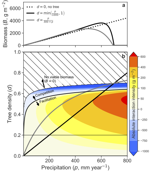
Figure S1a illustrates the transition from facilitation to competition for these two functional forms. Figure S1b shows the absolute interaction intensity in the (p,d) plane, and helps us interpret the graph on the top. When a dark curve in the bottom panel crosses the border between facilitation and competition, we see in the top panel that the dark curves cross the no-tree solution. For higher values of d, when the dark curves in the bottom panel cross into the no-viable-biomass zone, we also see a collapse of the vegetated solutions in the top panel. Finally, Fig. S1b helps us understand, from another point of view, why there cannot be a transition from facilitation to competition in the case of no carrying capacity and constant tree density, as will be shown in Supporting Information S2. Constant density solutions (see for example the dotted line at d=0.2) always cross from competition to facilitation as p increases, never the other way around. By changing tree density from a constant value to increasing functions of precipitation, as depicted by the solid dark lines, one can get the usual transition pattern of the SGH.
SI 2: Role of carrying capacity in the SGH patterns
We explore here the model results for each of the two mechanisms in the case where the logistic growth term is rendered inactive. This is achieved by taking the carrying capacity k\to\infty, which makes f_k(B) = \left(1 - B/k\right)\to 1. We can now find analytical expressions for the steady-state solutions of the model described in Equations (1) in the main paper. The nontrivial (B\neq0) steady-state solutions (B^\star,S^\star) read:
\begin{align*} S^\star &= \frac{m}{a f_a(d)} \tag{S2a}\\ B^\star &= \frac{p-f_r(S^\star,d) - q_s \left(S^\star\right)^c}{e_0f_e(d)S^\star} \tag{S2b} \end{align*}
These solutions are a typical instance of the R-star rule [S1], and from them we can express two important features:
- The steady-state resource level S^\star (generally called R^\star in consumer-resource modeling, therefore the name of the rule) is independent of the resource supply rate, p.
- The nontrivial (B\neq0) steady-state consumer level B^\star is linear in the resource input rate, p.
Figure S2 shows the steady-state biomass B^\star (top panels) and relative soil water content S^\star (bottom panels). The left and right columns correspond to the canopy mechanism and the root mechanism, respectively. A careful examination of the steady-state solutions teaches us that:
- For the canopy mechanism, 0\leq f_e(d) < f_a(d)<1 for any d>0 (see inset in Fig. S2c). From these facts it follows that the linear function for the positive tree-density solution (B^\star(p,d>0)) has a higher slope and a lower intercept1 than the no-tree solution (B^\star(p,d=0)). Because of its lower intercept, the positive density solution surpasses the zero-tree density solution from below (lower B). This means that eliminating the logistic growth term from the model described by the SGH: we have competition for p below the transition point, and facilitation for p above that point. Furthermore, for the parameter values we used here, the transition point occurs at extremely low values of p and B. Looking from `farther away’, the interactions appear facilitative for most of the precipitation gradient (Fig. S2a).
- For the root mechanism, two straight-line solutions B^\star always have the same slope, regardless of their d value, and therefore never intersect. The root mechanism can be either facilitative or competitive, depending on the soil water content (see inset in Fig. S2d). Figure S2b shows a scenario where the interaction is always facilitative. By changing the model parameters m,a,d (see Eq. S2a), one can also find higher soil water content levels that always yield competitive interactions.
The arguments above demonstrate that, whenever tree density is constant, the introduction of an additional growth-limiting factor that strengthens with increasing precipitation is a for the emergence of the transition described by the SGH.
SI 3: Transient dynamics
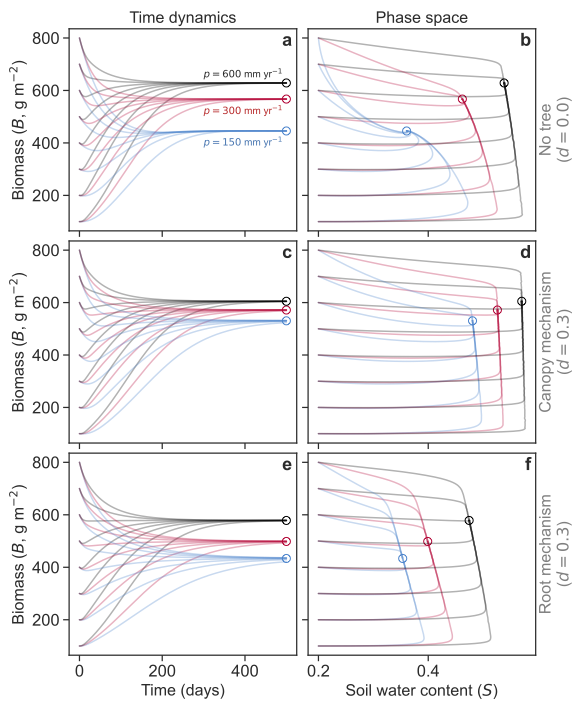
The typical timescale for the dynamics of herb biomass (B) is comparable to the length of the growing season used in this study, 180 days. Figure S3 shows the time dynamics (left column) and phase space (right column) for three precipitation levels (p=\{150,300,600\} mm year^{-1}) and three tree conditions: no tree (d=0, top row), canopy mechanism (d=0.3, middle row), and root mechanism (d=0.3, bottom row). Linear stability analysis of the numerically found steady-state solutions (hollow circles) reveals them to be stable nodes (real and negative eigenvalues).
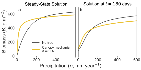
Crucially, the facilitation–to–competition switch persists when we examine transient dynamics, not only steady‐state outcomes. In Fig. S4, we compare the steady‐state pattern (panel a) with solutions obtained by integrating Eqs. (1) in the main text for 180 days (panel b). The qualitative result is the same in both cases, with positive tree effects at low precipitation and negative effects at high precipitation. Temporal dynamics, however, alter the details: the magnitude of facilitation and competition, and the precipitation at which the switch occurs, differ between transient and steady‐state results.
SI 4: Interaction intensity
As a rule, trees facilitate herb growth when their density is low and the system is under water stress (low p). Competition over water arises at high tree density values and under low water stress. Focusing on the canopy mechanism, Figure S5 shows that in the (p,d) parameter space, the boundary between facilitation and competition (solid black curve) follows a negative relation: as precipitation increases, a lower tree density is sufficient to shift the balance from facilitation to competition. This border is the same for both interaction intensities definitions, since zero interaction intensity means that the biomass solution with tree density (B_T) equals the biomass solution with no tree density (B_0). The area hatched in black at the top of both panels, where tree density is very high, indicates the region in the parameter space where there are only trivial (B=0) vegetated solutions.
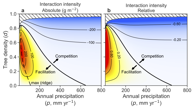
As shown in Fig. 3a in the main text, we can get unimodal curves when using the absolute interaction intensity. The dashed black curve in Fig. S5a shows the location of the local maxima in the (p,d) parameter space. To the left of this curve, the interaction intensity is positive and increases with precipitation. Once we cross this curve (from left to right), interaction intensity is still positive, but it decreases with precipitation. This ridge-like curve disappears when we use the relative interaction intensity instead: there is only monotonic decrease with precipitation.
SI 5: A deeper look into the model
In order to find useful ways of thinking about the model, we perform a non-dimensionalization of the equations. For our purposes, it makes more sense to describe the second equation as the rate of change of absolute soil water content W=nz_rS, instead of the equivalent nz_r\,dS/dt as shown in Eqs. (1) in the main text. Since the active soil layer nz_r has length dimension (z_r is the depth of the herb rooting zone, while the porosity n is non-dimensional), absolute soil water content W is also a length (it is commonly called soil water depth). Finally, we note that 1 millimeter of water is equivalent to 1 liter per meter squared, so reporting W as length is the same as volume per unit area. The full model equations now read:
\begin{align*} \frac{dB}{dt} &= a\, {f_a}(d)\, \left(1-\frac{B}{k}\right)B\, S - m\, B \tag{S3a} \\ \frac{dW}{dt} &= p - q_{s} S^c - e_0\, {f_e}(d) B\, S - {f_r}(S ,d). \tag{S3b} \end{align*}
The independent and dependent variables of this dynamical system have the following dimensions:
| Quantity | Symbol | Dimension | Units |
|---|---|---|---|
| Biomass density | B | density \rho | \text{g/m}^2 |
| Absolute soil water content | W | length L | \text{mm} |
| Time | t | time T | day |
Accounting for all the model parameters that have dimensions, we have eight: a,k,m,(nz_r),p,q_s,e_0,\lambda. (Here we treat nz_r as a single parameter.) The parameter \lambda appears inside the function f_r(S,d). All of these parameters have dimensions that derive from the three basic ones shown in the table. According to Buckingham’s \Pi Theorem, when performing non-dimensionalization of the equations, the number of independent dimensionless groups is equal to the number of dimensional parameters minus the number of fundamental dimensions. Since we have 8 dimensional parameters and 3 fundamental dimensions (biomass density, length, and time), we obtain 8-3=5. In simple terms, although the model contains eight dimensional parameters, its behavior can be fully captured by just five independent dimensionless combinations.
We start now the non-dimensionalization process by defining the following new non-dimensional variables:
\begin{align*} \text{non-dimensional biomass}&& \tilde{b} &= B/\xi_1 % \frac{B}{\xi_1} \tag{S4a}\\ \text{non-dimensional time}&& \tilde{t} &= t/\xi_2. \tag{S4b} \\ \text{non-dimensional water}&& S &= W/\xi_3. \tag{S4c} \end{align*}
We have many choices for \xi_1,\xi_2,\xi_3. A suitable choice here is
\begin{align*} \xi_1 &= \frac{a}{e_0} \tag{S5a} \\ \xi_2 &= \frac{1}{a} \tag{S5b}\\ \xi_3 &= nz_r. \tag{S5c} \end{align*}
Substituting Eqs. S4 and S5 into Eqs. S3 yields the non-dimensional dynamical system:
\begin{align*} \frac{d\tilde{b}}{d\tilde{t}} &= {f_a}(d)\, \left(1-\frac{\tilde{b}}{\tilde{k}}\right)\tilde{b}\, S - \tilde{m}\,\tilde{b} \tag{S6a} \\ \frac{dS}{d\tilde{t}} &= \tilde{p} - \tilde{q}_{s} S^c - {f_e}(d) \tilde{b} S - \tilde{f}_r(S ,d). \tag{S6b} \end{align*}
As we can see, this choice of \xi_1,\xi_2,\xi_3 leaves us a non-dimensional system, where every single variable, parameter, term or function is dimensionless. For this specific choice of \xi scaling factors, we have a system with unity growth rate and unity maximum evapotranspiration rate.
The non-dimensional parameters (\Pi parameters) for the equations above are:
\begin{align*} \text{non-dimensional herb mortality rate },\Pi_1&& \tilde{m} &= \frac{m}{a} \tag{S7a}\\ \text{non-dimensional carrying capacity },\Pi_2&& \tilde{k} &= \frac{k}{a/e_0} \tag{S7b}\\ \text{non-dimensional precipitation rate },\Pi_3&& \tilde{p} &= \frac{p}{anz_r} \tag{S7c}\\ \text{non-dimensional sat.\ hyd.\ cond. },\Pi_4&& \tilde{q}_s &= \frac{q_s}{anz_r} \tag{S7d}\\ \text{non-dimensional tree-root hydraulic rate },\Pi_5&& \tilde{\lambda} &= \frac{\lambda}{anz_r} \tag{S7e} \end{align*}
This exercise is instrumental in shedding light on the impact of various model parameters on its behavior:
- The active soil layer n z_r (mm), where n is soil porosity (dimensionless) and z_r is the rooting depth of herbs (mm), sets the maximum volume of water that can be stored and made available to herbs. As Eqs. (1) in the main text indicate, n z_r can only impact the transient dynamics of (B,S), never their steady-state solutions. Of course, due to the third conversion in Eq. S4, n z_r rescales S into W=nz_rS.
- The denominator a n z_r represents a characteristic water throughput, where a sets the characteristic timescale and nz_r is the volume of water per unit area (1 mm = 1 L mm^{-2}). It sets the scale for precipitation, drainage, and root uptake/uplift (\tilde{p},\tilde{q}_s,\tilde{\lambda}): higher values correspond to processes faster than the characteristic resource throughput in the system.
- The ratio (a/e_0) naturally emerges as a water-use efficiency, converting herb water uptake into biomass production. In fact, when tree density is zero (d=0) and herb biomass is low (so that 1-\tilde{b}/\tilde{k}\approx1), the evapotranspiration loss term in Eq. S6b is identical to the biomass growth term in Eq. S6a. This symmetry highlights the direct coupling of growth and water loss. The conversion dictated by S4a means that whatever the non-dimensional steady state \tilde{b} one gets by solving Eqs. S6, we divide it by the water-use efficiency a/e_0 to get the dimensional biomass B.
- The typical growth timescale 1/a acts as a fundamental clock for all other remaining parameters (see S7).
- \tilde{k} shows how the dimensional carrying capacity k is rescaled by water-use efficiency a/e_0. This helps us understand that the logistic term is weaker (meaning that water is the main limiting factor) for either large k or low water-use efficiency a/e_0.
SI 6: Logistic growth extension: effective herb–herb interactions
In the main text, the logistic term is introduced as a phenomenological representation of density-dependent limitation of herb growth. In Section S9, we will show that such a term can arise mechanistically from nutrient limitation. Here, we provide an alternative interpretation in which density dependence emerges from unresolved interactions within a diverse herbaceous community.
We consider a community composed of multiple herb species with biomass B_i (i=1,\dots,n), each interacting with soil water S. A standard representation of competitive interactions is given by a Lotka–Volterra-type system:
\begin{align*} \frac{dB_i}{dt} &= a_i\, {f_a}(d)\, B_i\, S \left(1 - \sum_{j=1}^n \alpha_{ij} B_j \right) - m_i B_i, \tag{s8a}\\ n z_r\frac{dS}{dt} &= p - e_0\, {f_e}(d) \left(\sum_{i=1}^n B_i\right) S - {f_r}(S ,d) - q_{s} S^c, \tag{s8b} \end{align*}
where \alpha_{ij} represents the effect of species j on species i, capturing competition for non-water resources such as nutrients or space.
We define the total herb biomass as: \begin{equation} B = \sum_{i=1}^n B_i. \tag{S9} \end{equation}
Summing Equation S8a over all species yields: \begin{equation} \frac{dB}{dt} = \sum_{i=1}^n a_i\, {f_a}(d)\, B_i\, S - \sum_{i=1}^n m_i B_i - \sum_{i=1}^n a_i\, {f_a}(d)\, B_i\, S \sum_{j=1}^n \alpha_{ij} B_j. \tag{S10} \end{equation}
At this stage, the dynamics of B are not closed, as they depend on the full distribution of species biomasses and interaction coefficients. To obtain a tractable expression, we introduce a mean-field approximation. Specifically, we assume that species are sufficiently similar in their growth and interaction parameters such that:
\begin{equation} a_i \approx a, \qquad m_i \approx m, \qquad \alpha_{ij} \approx \bar{\alpha}. \tag{S11} \end{equation}
Under these assumptions, the above equation simplifies to:
\begin{equation} \frac{dB}{dt} \approx a\, {f_a}(d)\, S \sum_{i=1}^n B_i - m B - a\, {f_a}(d)\, S\, \bar{\alpha} \sum_{i=1}^n \sum_{j=1}^n B_i B_j. \tag{S12} \end{equation}
Using the identity \sum_{i,j} B_i B_j = \left(\sum_i B_i\right)^2 = B^2, we obtain:
\begin{equation} \frac{dB}{dt} \approx a\, {f_a}(d)\, B S - m B - a\, {f_a}(d)\, S\, \bar{\alpha} B^2. \tag{S13} \end{equation}
This can be rewritten in logistic form:
\begin{equation} \frac{dB}{dt} = a\, {f_a}(d)\, B \left(1 - \frac{B}{k}\right) S - m B, \tag{S14} \end{equation}
where the effective carrying capacity is given by k = 1/\bar{\alpha}.
Thus, a quadratic saturation term in total herb biomass emerges naturally from pairwise competitive interactions when these are aggregated and approximated at the community level.
This derivation shows that logistic-type density dependence can arise as an effective description of herb–herb interactions when species-level details are not resolved. However, several important caveats apply.
First, the mean-field approximation assumes that species are sufficiently similar in their growth rates and interaction strengths. In real herbaceous communities, species often differ substantially in functional traits and resource-use strategies. As a result, competitive interactions may be highly structured rather than homogeneous.
Second, the aggregation of species into a single biomass variable eliminates information about community composition, species richness, and trait variation. In particular, competitive effects that manifest as changes in species composition or diversity (e.g., shifts in dominance or richness decline) may not translate into a reduction in total biomass and are therefore not captured by the logistic term.
Third, the quadratic term represents the net effect of all pairwise interactions and should be interpreted as a phenomenological closure rather than a mechanistic representation of specific competitive processes.
Accordingly, in the main text, the herb biomass variable could be interpreted as an aggregated herbaceous compartment, and the logistic term as an effective density-dependent limitation that may arise from unresolved competition, crowding, or other non-water resource constraints. Explicit representation of multiple herb species or functional types would be required to capture compositional dynamics and trait-dependent responses.
SI 7: A gradient of evaporative demand
Here, we demonstrate that our model can produce a transition from facilitation to competition, not only along a precipitation gradient but also across an evaporative demand gradient (Figure S6).
SI 8: Choosing the Right Resource Metric for the SGH
The Stress Gradient Hypothesis (SGH) predicts a shift from facilitation to competition as a resource increases. A critical question is which resource metric to use: resource supply rate (like precipitation) or resource abundance (like soil water content). We demonstrate here that the resource supply rate is the appropriate metric for assessing the SGH.
When we analyze our model using precipitation as the control parameter (x-axis in a B vs. p plot), the results clearly demonstrate the SGH pattern. For both the canopy and root mechanisms, we observe a transition from positive to negative tree-herb interactions as precipitation increases, mirroring field observations.
In contrast, if we use soil water content as the resource metric, the SGH pattern vanishes. Figure S7 shows the same herb biomass solutions as Figure 2 in the main text, but plotted against soil water content.
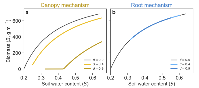
The nontrivial (B\neq 0) solutions can be readily obtained by equating Eqs.~(1) in the main text to zero and solving for B:
\begin{align*} \text{Canopy mechanism: } B^\star(S) &= k\left(1-\frac{m}{aSf_a(d)}\right) \tag{S15a} \\ \text{Root mechanism: } B^\star(S) &= k\left(1-\frac{m}{aS}\right) \tag{S15b} \end{align*}
From these solutions we learn:
- Canopy mechanism: Because f_a(d>0)<f_a(d=0), the steady-state herb biomass with trees (B_T) is always lower than the biomass without trees (B_0). Trees always reduce light, which directly suppresses herb growth. Because the facilitative effect of water conservation is no longer a factor, the interaction intensity is always negative (competitive).
- Root mechanism: Herb biomass becomes completely independent of tree density (it lacks the variable d). Trees influence herbs solely by altering soil water levels, so if that level is fixed, the trees have no effect. The interaction intensity is always zero.
This result, that the SGH pattern disappears when using soil water content as the metric, occurs for a fundamental reason: soil water content, unlike precipitation, is an intrinsic property of the ecosystem, not an external force. It is the result of multiple processes such as rainfall, evapotranspiration, drainage, etc; all of which interact with the tree’s presence to determine the final soil water content. By holding soil water constant, we are artificially decoupling the very mechanisms that create the SGH pattern. Therefore, using resource abundance (soil water content) as the metric of stress renders the SGH meaningless within this mechanistic framework, as it nullifies the resource component in our consumer-resource model.
The resource supply rate (precipitation) is the external driver of the system’s state, making it the correct measure of abiotic stress for a resource-based SGH. It allows us to capture the full interplay of facilitative and competitive forces that are the core of the hypothesis.
SI 9: Logistic growth extension: nutrient-limited growth
To justify our choice of introducing a limiting factor to herb growth as a logistic term, we do the exercise of explicitly introducing a new essential resource, a nutrient N. Our model can be extended to include the nutrient dynamics as follows:
\begin{align*} \frac{dB}{dt} &= a\, {f_a}(d)\, B\, N\,S - m\, B \tag{S16a}\\ n z_r\frac{dS}{dt} &= p - e_0\, {f_e}(d) B\, S - {f_r}(S ,d) - q_{s} S^c \tag{S16b} \\ \frac{dN}{dt} &= N_\text{in} -\mu N B - \nu N.\tag{S16c} \end{align*}
The first equation, S16a, describes the herb biomass dynamics, where we have replaced our original logistic term f_k(B) with a nutrient term, N. Equation S16c describes the nutrient’s dynamics, where it is introduced at a constant rate N_\text{in}, consumed by herbs (at a rate proportional to both herb biomass and nutrient availability, \mu NB), and lost from the system at a rate proportional to its own abundance, \nu N.
We now assume that the nutrient dynamics are much faster than those of the herb biomass (B) and soil water (S). We can therefore perform an adiabatic elimination by setting the rate of change of the nutrient to zero to find its quasi-steady-state:
\begin{align*} 0 &= N_\text{in} -\mu N B - \nu N \tag{S17a}\\ \implies N^\star &= \frac{N_\text{in}}{\nu}\frac{1}{\frac{\mu}{\nu}B+1}, \tag{S17b} \end{align*}
where N^\star denotes the quasi-steady-state nutrient concentration. Substituting N^\star into the herb biomass equation gives:
\begin{equation} \frac{dB}{dt} = a\, \frac{N_\text{in}}{\nu} {f_a}(d)\, B\left( \frac{1}{\frac{\mu}{\nu}B+1} \right) S - m\, B. \tag{S18} \end{equation}
The term in the parenthesis acts as a saturating function of B. When herb biomass is low, the term is close to one, and as biomass increases, the function decreases, effectively slowing the growth rate. This plays the same role as the logistic term we assumed in the main text.
To derive the exact logistic form, we can make an additional assumption. If we assume that the herbs are highly inefficient at consuming the nutrient relative to its decay rate (\mu\ll\nu), we can use a first-order Taylor series expansion:
\begin{equation} \frac{1}{\frac{\mu}{\nu}B+1} \approx 1 - \frac{\mu}{\nu}B . \tag{S19} \end{equation}
Substituting this approximation into the herb biomass equation now reveals a classic logistic term:
\begin{equation} \frac{dB}{dt} = a\, \frac{N_\text{in}}{\nu} {f_a}(d)\, B\left( 1 - \frac{B}{k} \right) S - m\, B, \tag{S20} \end{equation}
where the carrying capacity can be identified with k=\nu/\mu. If the factor N_\text{in}/\nu is then incorporated into a, we get exactly Equation (1a) in the main text.
S10: Combined canopy and root mechanisms
The combined model activates both the canopy shading terms and the root water function in Eq. (1) in the main text. No additional parameters are required: the canopy functions f_a(d) and f_e(d) reduce herb assimilation and evapotranspiration, while the root term f_r(S, d) acts concurrently on the soil water balance.
We first examine the combination of two of the most common mechanisms: canopy shading and competitive water uptake alone, setting hydraulic lift to zero (\lambda_h = 0, Fig. S8c). Even in this conservative case, combining the two mechanisms still produces net facilitation at low precipitation (Fig. S8a): the facilitative benefit of shading outweighs the competitive cost of root water uptake. Adding root competition narrows the facilitation window relative to the canopy-only model and shifts the transition point to lower rainfall, but does not eliminate facilitation.
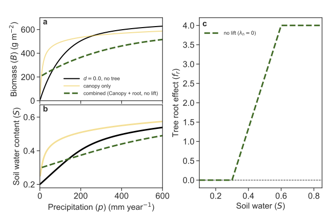
Introducing hydraulic redistribution (\lambda_h > 0) changes the outcome in a density-dependent way, see Fig. S9. At moderate tree density (d = 0.4), facilitation at low rainfall is preserved and the SGH transition is reproduced. At high tree density (d = 0.8), competition dominates across the entire precipitation range.
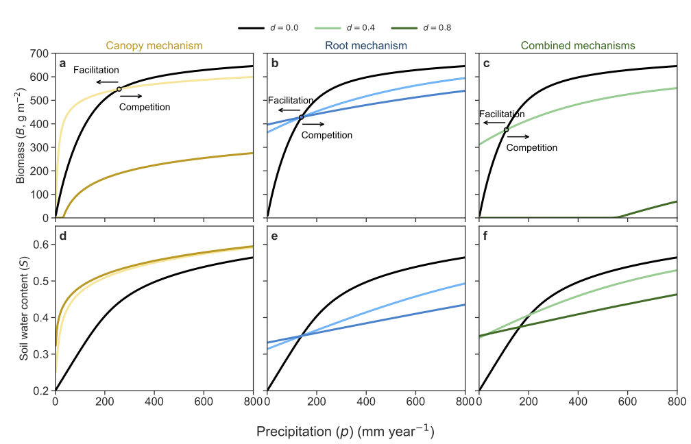
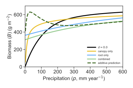
The combined model is sub-additive, see Fig. S10. The actual joint biomass falls below the additive prediction (B_\mathrm{additive} = B_\mathrm{canopy} + B_\mathrm{root} - B_\mathrm{baseline}) across the entire gradient, and the additive prediction substantially overestimates facilitation at low precipitation. This sub-additivity arises because the two mechanisms share the same soil water pool: canopy shading conserves water by reducing evapotranspiration, but this conserved water remains accessible to root uptake, partially offsetting the facilitative benefit of shading and amplifying competition.
SI 11: Infiltration
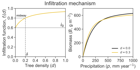
The infiltration mechanism is a variation of the canopy mechanism. In both, canopy shading reduces herb assimilation through f_a(d); here, however, the facilitative pathway is not a reduction in evapotranspiration but an increase in effective infiltration as tree density rises. The model therefore keeps the growth-side shading term and replaces the rainfall input with an infiltrated input p\,f_i(d):
\begin{align*} \frac{dB}{dt} &= a\,f_a(d)\,\Bigl(1-\frac{B}{k}\Bigr) B\,S \;-\; m\,B, \tag{S21a}\\ n z_r\,\frac{dS}{dt} &= p\,f_i(d) \;-\; q_{s}\,S^c \;-\; e_0\,B\,S , \tag{S21b} \end{align*}
The infiltration factor f_i(d) follows [S2]: \begin{equation} f_i(d) \;=\; \frac{d+i_0\,\delta}{d+\delta}, \tag{S22} \end{equation}
so that f_i(0)=i_0 (minimum infiltration without trees) and f_i(d)\to 1 as d increases; see Fig. S11a. The parameter \delta sets the density scale at which f_i is midway between i_0 and 1. Figure S11b shows the SGH transition for the infiltration mechanism.
This relationship captures two possible processes. The first is that canopy shading can suppress biological soil crusts (biocrusts), which often form a hardened surface layer that reduces infiltration. The second process is the compaction of the surface by the mechanical impact of rain drops, which also reduces infiltration. As tree density increases, the canopy limits biocrust activity and protects the surface from direct rain drop impacts, thus allowing more water to infiltrate into the soil, and increasing the effective water supply to herbs.
SI 12: Parameter values and their ecological basis
The model parameters in Table 1 in the main text represent a generalized dryland ecosystem rather than a specific site. Where possible, the values and ranges were chosen to be consistent with published measurements from drylands; some parameters are modelling choices set to produce ecologically realistic order-of-magnitude behaviour rather than values derived from a single measurement, because direct measurements of these quantities are not available in the literature. Below we describe how each cited value connects to its source.
Model state variables
The state variable B is the herbaceous biomass density (gram per meter squared). Annual live aboveground biomass across dryland sites is predominantly in the range 0–1000 gram per meter squared [S3] (Fig. 4 therein), and the model’s carrying capacity keeps the biomass output in this range.
The state variable S \in [0, 1] is the relative soil water content, defined as the ratio of volumetric water content to total pore volume [S4]. S = 0 corresponds to completely dry soil and S = 1 to saturation; these bounds are set by physical constraints.
Tree cover range
The parameter d \in [0,1] represents woody plant canopy density; it is treated as a fixed environmental parameter over which model outcomes are evaluated, rather than a dynamical variable.
Soil hydraulic parameters
The soil hydraulic parameters are chosen to be consistent with the range of values tabulated in [S4] for sandy to loam soils (Table 2.1 therein). The saturated hydraulic conductivity q_{sat} = 800 mm per day (= 80 cm per day) matches the sandy loam value in that table (K_s \approx 80 cm per day). The porosity n = 0.4 is close to the loamy sand and sandy loam values (n = 0.42–0.43). The field capacity S_{fc} = 0.6 falls between the sandy loam (s_{fc} = 0.56) and loam (s_{fc} = 0.65) entries. The drainage exponent c = 10 is of the same order as the sandy soil range in Table 2.1 (c = 11–13). The herb rooting depth z_r = 300 mm falls at the shallow end of the range used for illustrative examples in [S4] (Z_r = 30–90 cm; Fig. 2.7 therein) and is representative of the effective root zone of dryland herbaceous grasses. The model uses a simplified two-threshold soil moisture balance with a single lower threshold S_h = 0.3 below which evapotranspiration is zero; this value is comparable to the stomatal-closure threshold s^\star = 0.31 reported for loamy sand in Table 2.1, and reflects the effective lower limit of plant-available water in a sandy dryland soil.
Precipitation range
Drylands can be defined using various criteria, including temperature, climate classification, or aridity indices. Here we follow [S5], who characterize drylands as regions with an annual precipitation of \approx 600 mm per year; our precipitation range p = 0–600 mm per year therefore covers dryland climates well, from hyperarid deserts at the lower end to dry-subhumid conditions where grass–tree savannas are common at the upper end. In the model, precipitation above this threshold is sufficient to maintain soil moisture above the stress threshold, so that water ceases to be the primary limiting factor.
Assimilation rate
In the biomass equation, the assimilation rate a corresponds to the intrinsic per-capita growth rate at low biomass, equivalent to the relative growth rate (RGR) of well-watered seedlings. [S6] report RGR values of 0.04–0.15 g g d^{-1} across twelve native rangeland forb species; our value of a = 0.05 d^{-1} falls at the lower end of this range, appropriate for slower-growing, dryland-adapted herbaceous vegetation.
Carrying capacity and mortality
The carrying capacity k = 1000 gram per meter squared equals the upper bound of the observed biomass range. Ecologically, k represents the maximum standing biomass supported once water and light are non-limiting, i.e., constrained by nutrients or other factors (see also Section S9). The mortality rate m = 0.01 d^{-1} implies a biomass turnover timescale of approximately 100 d, consistent with the growing-season lifespan of annual dryland grasses and the typical decay rates measured for dryland herbaceous biomass.
Evapotranspiration rate per unit biomass
The parameter e_0 = 0.005 mm d^{-1} / g m^{-2} is the maximum evapotranspiration rate per unit herb biomass density. Because no single source directly reports this quantity in the units used by the model, we derived it from two more commonly reported quantities: biomass-level water-use efficiency and the rate of biomass production.
The available empirical information is usually reported as water-use efficiency, or transpiration efficiency, in units of gram biomass produced per kg water transpired. This quantity describes how much biomass is produced per amount of water used, but it does not by itself contain a time dimension. To convert it into a daily evapotranspiration rate, we also need the daily rate at which biomass is produced. In the model, the assimilation rate a corresponds to the relative growth rate of herbaceous biomass under non-limiting conditions, while m represents biomass loss through mortality. Thus, the net rate of biomass increase is a-m = 0.05 - 0.01 = 0.04 d^{-1}.
For a given herb biomass density B (g m^{-2}), the net daily biomass production is therefore (a-m)B, with units of g m^{-2} d^{-1}. Dividing this biomass production rate by water-use efficiency converts biomass production into the amount of water required to support that production. Reported transpiration efficiency values for wheat, a C3 species, are approximately in the range of 4–12 g/kg [S7][S8]. We therefore used an intermediate value of 8 g/kg.
With these units, dividing g m^{-2} d^{-1} by g/kg gives kg m^{-2} d^{-1}. This is easily converted to the model’s water-depth units because a water depth of 1 mm over 1 m^2 corresponds to 1 kg of water. Thus, kg m^{-2} d^{-1} is equivalent to mm d^{-1}. The biomass-specific evapotranspiration coefficient is therefore obtained by dividing the net daily biomass production rate by water-use efficiency and expressing the result per unit standing biomass:
\begin{equation*} e_0 = \frac{a-m}{\mathrm{WUE}} = \frac{0.04 \text{ d} ^{-1}}{8 \text{ g kg}^{-1}} = 0.005 \text{mm d}^{-1}/\text{ g m}^{-2}. \end{equation*}
Shading function exponents
The shading functions f_a(d) = (1-d)^{\beta_a} and f_e(d) = (1-d)^{\beta_e} were chosen as simple nonlinear functions that continuously interpolate between no shading (d=0) and full canopy (d=1). Analysis of the model shows that \beta_e > \beta_a is a necessary condition for the facilitation-to-competition transition: transpiration must be more sensitive to shading than assimilation (Results Section in the main text). This modelling requirement is qualitatively supported by empirical evidence. Experimental measurements on grapevines under mild shading (8% shade cloth) show that leaf transpiration is significantly reduced (\approx 25%) while net CO_2 assimilation is statistically unaffected [S9]. Path analyses for poplar trees show that the standardized effect of PAR reduction on transpiration (path coefficient \approx 0.57) is substantially larger than its effect on photosynthesis (\approx 0.37) [S10]. Across many subtropical fruit species and shade intensities, shading consistently improves plant water-use efficiency, implying that transpiration losses are reduced proportionally more than carbon assimilation [S11]. The specific exponents \beta_a = 1/3 and \beta_e = 4 are modelling choices that satisfy this inequality and yield ecologically plausible shading curves; at d = 0.5, for example, f_a \approx 0.79 while f_e \approx 0.06, reflecting that a moderate canopy barely affects herb assimilation yet substantially suppresses transpiration.
Tree water uptake and hydraulic redistribution
The parameter \lambda_{fc} = 10 mm d^{-1} is the maximum rate at which trees uptake soil water (attained at field capacity and full tree density d = 1). [S12] measured daily evapotranspiration of dense stands, reporting a daily average of {\approx 3.7} mm d^{-1} with peak values approaching {\approx 9.5} mm d^{-1} during the growing season. Our value \lambda_{fc} = 10 mm d^{-1} represents the upper physiological demand attained at full tree density and field capacity soil moisture.
The parameter \lambda_h = -2 mm d^{-1} sets the maximum rate of hydraulic redistribution, whereby trees add water to the shallow soil layer. The negative sign indicates a net water subsidy to the herb rooting zone. Field measurements across semi-arid systems report hydraulic redistribution fluxes of 0.04–1.3 mm d^{-1} (empirical) and 0.1–3.23mm d^{-1} (modeling estimates) [S13]; |\lambda_h| = 2 mm d^{-1} therefore falls within the upper range of observed and modeled values.
In our model, both parameters in most cases do not attain their maximum values: tree water uptake is maximized at field capacity (S = S_{fc}), while hydraulic redistribution is maximized at the lower threshold (S = S_h); under typical fluctuating dryland soil moisture, neither extreme is sustained.
SI references
S1.
D. Tilman, Resource Competition and Community Structure, Monographs in Population Biology (Princeton University Press, Princeton, NJ, 1982), vol. 17.
S2.
Gilad, E., Von Hardenberg, J., Provenzale, A., Shachak, M., & Meron, E. (2004). Ecosystem engineers: from pattern formation to habitat creation. Physical review letters, 93(9), 098105.
S3.
MacDougall, A. S., Esch, E., Chen, Q., Carroll, O., Bonner, C., Ohlert, T., … & Seabloom, E. W. (2024). Widening global variability in grassland biomass since the 1980s. Nature ecology & evolution, 8(10), 1877-1888.
S4.
Rodriguez-Iturbe, I., Porporato, A., Laio, F., & Ridolfi, L. (2001). Plants in water-controlled ecosystems: active role in hydrologic processes and response to water stress: I. Scope and general outline. Advances in Water Resources, 24(7), 695-705.
S5.
Huang, J., Yu, H., Dai, A., Wei, Y., & Kang, L. (2017). Drylands face potential threat under 2 C global warming target. Nature Climate Change, 7(6), 417-422.
S6.
James, J. J., & Drenovsky, R. E. (2007). A basis for relative growth rate differences between native and invasive forb seedlings. Rangeland ecology & management, 60(4), 395-400.
S7.
Fletcher, A., Christopher, J., Hunter, M., Rebetzke, G., & Chenu, K. (2018). A low-cost method to rapidly and accurately screen for transpiration efficiency in wheat. Plant Methods, 14(1), 77.
S8.
Qiao, Y., Li, D., Qiao, W., Li, Y., Yang, H., Liu, W., … & Dong, B. (2022). Development and application of a relative soil water content–transpiration efficiency curve for screening high water use efficiency wheat cultivars. Frontiers in Plant Science, 13, 967210.
S9.
Gutiérrez-Gamboa, G., Villalobos-Soublett, E., Garrido-Salinas, M., & Verdugo-Vásquez, N. (2024). Monofilament shading nets improved water use efficiency on high-temperature days in grapevines subjected to hyperarid conditions. Horticulturae, 10(2), 176.
S10.
Wang, B., Wang, Z., Wang, C., Wang, X., Jia, Z., & Liu, L. (2024). Elevated aerosol enhances plant water‐use efficiency by increasing carbon uptake while reducing water loss. New Phytologist, 243(2), 567-579.
S11.
Mditshwa, A., Magwaza, L. S., & Tesfay, S. Z. (2019). Shade netting on subtropical fruit: Effect on environmental conditions, tree physiology and fruit quality. Scientia Horticulturae, 256, 108556.
S12.
Shiferaw, H., Alamirew, T., Dzikiti, S., Bewket, W., Zeleke, G., & Schaffner, U. (2021). Water use of Prosopis juliflora and its impacts on catchment water budget and rural livelihoods in Afar Region, Ethiopia. Scientific reports, 11(1), 2688.
S13.
Neumann, R. B., & Cardon, Z. G. (2012). The magnitude of hydraulic redistribution by plant roots: a review and synthesis of empirical and modeling studies. New Phytologist, 194(2), 337-352.
Footnotes
Slope \sigma: for d=0 the slope is \sigma_{0}=a/(e_0m), whereas for d>0 it is \sigma_d=\sigma_0 \cdot (f_a(d)/f_e(d)). Since f_a(d)>f_e(d), we have that \sigma_d>\sigma_0.
Intercept \omega: for d=0 the intercept is \omega_0=-(q_s/e_0)(m/a)^{c-1}, whereas for d>0 it is \omega_d=\omega_0(1/f_e(d))(1/f_a^{c-1}(d)). Since f_a(d),f_e(d)<1 and c>2, we have that each of the parenthesis in the expression for \omega_d is greater than 1, and therefore \omega_d<\omega_0 (remember the minus sign in \omega_0).↩︎