reactivity

question

What happens to a system when we perturb it slightly away from its stable equilibrium?

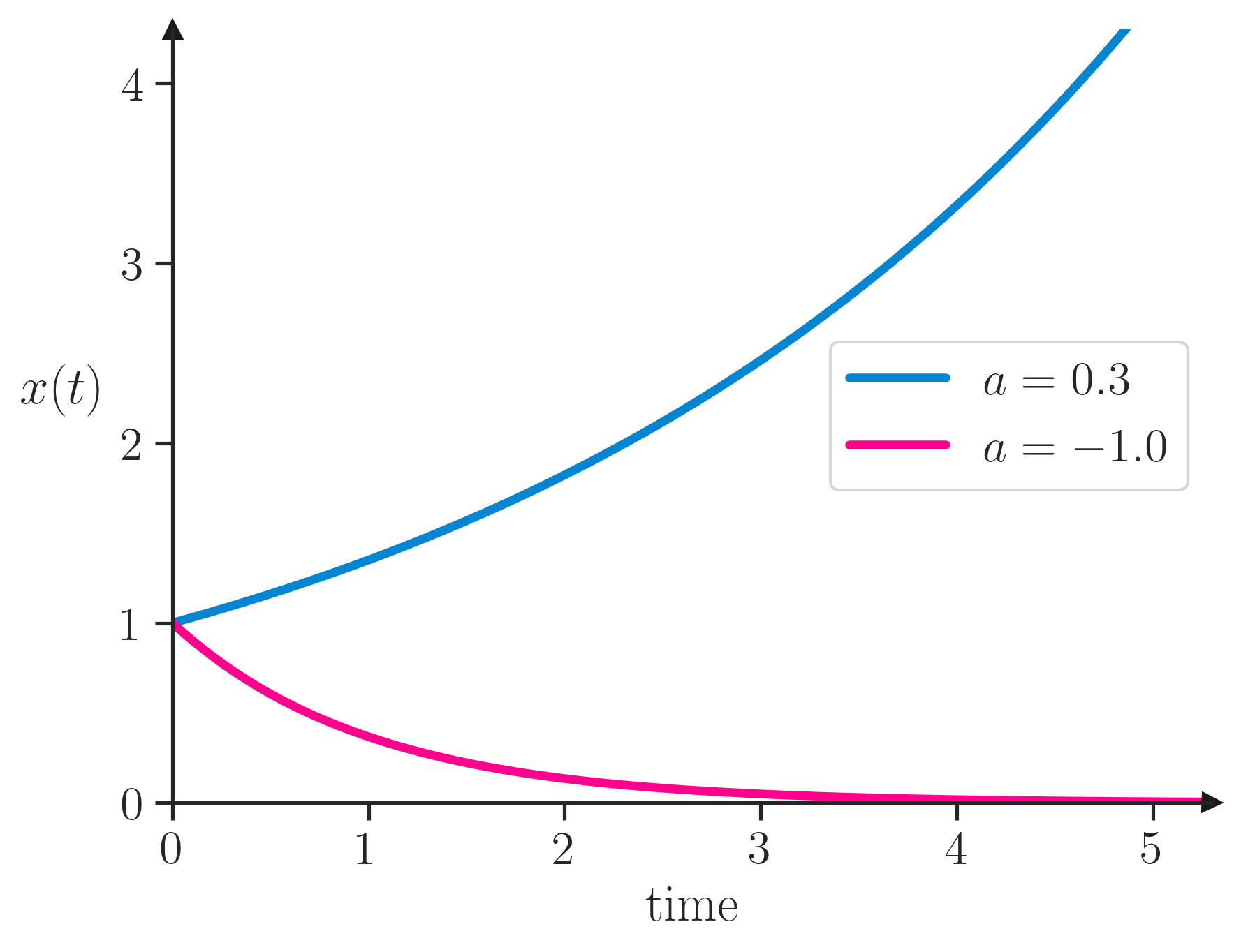
a 1d linear dynamical system

\[ \frac{dx}{dt} = ax. \]

\(x=0\) is a steady state solution. If we start away from it at \(x_0\), the solution can be obtained by integrating the equation above:

\[ x(t) = x_0 \,e^{at} \]

import numpy as np
import pandas as pd
import matplotlib.pyplot as plt
import matplotlib
import matplotlib.gridspec as gridspec
from scipy.integrate import solve_ivp
import seaborn as sns
sns.set_theme(style="ticks", font_scale=1.5)  # white graphs, with large and legible letters
# %matplotlib widget

def equation_1d(a, x):
    return [a * x]

# parameters as a dictionary
a1 = -1.0
a2 = +0.3

tmax=6
dt=0.01
x0 = 1.0
t_eval = np.arange(0, tmax, dt)

# solve the system

sol1 = solve_ivp(lambda t, y: equation_1d(a1, y),
                 [0, tmax], [x0], t_eval=t_eval)
sol2 = solve_ivp(lambda t, y: equation_1d(a2, y),
                 [0, tmax], [x0], t_eval=t_eval)

# learn how to configure:
# http://matplotlib.sourceforge.net/users/customizing.html
params = {
          'font.family': 'serif',
          'ps.usedistiller': 'xpdf',
          'text.usetex': True,
          # include here any neede package for latex
          'text.latex.preamble': r'\usepackage{amsmath}',
          'figure.dpi': 300
          }
plt.rcParams.update(params)
# matplotlib.rcParams['text.latex.preamble'] = [
#     r'\usepackage{amsmath}',
#     r'\usepackage{mathtools}']

fig, ax = plt.subplots()

bright_color1 = "xkcd:hot pink"
bright_color2 = "xkcd:cerulean"

ax.plot(sol2.t, sol2.y[0], color=bright_color2, lw=3, label=f'$a={a2}$')
ax.plot(sol1.t, sol1.y[0], color=bright_color1, lw=3, label=f'$a={a1}$')


ax.legend(loc='center right')
ax.set(xlim=[0,5.3],
       ylim=[0,4.3],
       xlabel='time',)
ax.set_ylabel(r'$x(t)$', labelpad=20, rotation=0)
# only left and bottom spines
ax.spines['right'].set_color('none')
ax.spines['top'].set_color('none')

ax.plot(1, 0, ">k", transform=ax.get_yaxis_transform(), clip_on=False)
ax.plot(0, 1, "^k", transform=ax.get_xaxis_transform(), clip_on=False)

the simplest 2d dynamical system

Let’s see what happens when we perturb a 2d linear dynamical system slightly away from its stable equilibrium.

\[\begin{align*} \frac{dx_1}{dt} &= ax_1 + bx_2 \\ \frac{dx_2}{dt} &= cx_1 + dx_2 \end{align*}\]

…or in matrix form:

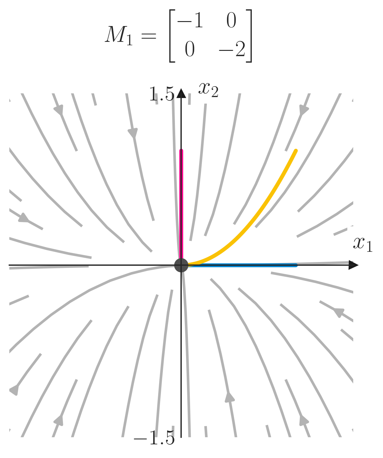
\[ \frac{d\mathbf{x}}{dt} = M \mathbf{x}, \] where \(\mathbf{x}=(x_1,x_2)\) and \(M = \begin{pmatrix} a & b \\ c & d \end{pmatrix}\).

The steady state solution is \(\mathbf{x}=(0,0)\). Let’s see the flow in this 2d space.

def system_equations_2d(p, x, y):
    return [p['a'] * x + p['b'] * y,
            p['c'] * x + p['d'] * y,
           ]

# parameters as a dictionary
A0 = {'a': -1.0, 'b': +0.0,
      'c': +0.0, 'd': -2.0}
A1 = {'a': -1.0, 'b': +1.0,
      'c': +0.0, 'd': -2.0}
A2 = {'a': -1.0, 'b': +10,
      'c': +0.0, 'd': -2.0}

min_x, max_x = [-3, 3]
min_y, max_y = [-3, 3]
div = 50
X, Y = np.meshgrid(np.linspace(min_x, max_x, div),
                   np.linspace(min_y, max_y, div))

# given initial conditions (x0,y0), simulate the trajectory of the system as ivp
def simulate_trajectory(p, x0, y0, tmax=10, dt=0.01):
    t_eval = np.arange(0, tmax, dt)
    sol = solve_ivp(lambda t, y: system_equations_2d(p, y[0], y[1]),
                    [0, tmax], [x0, y0], t_eval=t_eval)
    return sol

t0a = simulate_trajectory(A0, 0, 1, 100)
t0b = simulate_trajectory(A0, 1, 0, 100)
t0c = simulate_trajectory(A0, 1, 1, 100)
t1 = simulate_trajectory(A1, 0, 1, 100)
t2 = simulate_trajectory(A2, 0, 1, 100)

fig, ax = plt.subplots()

density = 2 * [1.0]
minlength = 0.05
arrow_color = 3 * [0.7]
bright_color1 = "xkcd:hot pink"
bright_color2 = "xkcd:cerulean"
bright_color3 = "xkcd:goldenrod"

# make sure that each axes is square
ax.set_aspect('equal', 'box')
ax.streamplot(X, Y, system_equations_2d(A0, X, Y)[0], system_equations_2d(A0, X, Y)[1],
              density=density, color=arrow_color, arrowsize=1.5,
              linewidth=2,
              minlength=minlength,
              zorder=-10
              )
ax.plot(t0a.y[0], t0a.y[1], color=bright_color1, lw=3)
ax.plot(t0b.y[0], t0b.y[1], color=bright_color2, lw=3)
ax.plot(t0c.y[0], t0c.y[1], color=bright_color3, lw=3)
ax.plot(t1.y[0][-1], t1.y[1][-1], 'o', color=3*[0.3], markersize=10)


# make spines at the origin, put arrow at the end of the axis
ax_list = [ax]
for axx in ax_list:
    axx.spines['left'].set_position('zero')
    axx.spines['bottom'].set_position('zero')
    axx.spines['right'].set_color('none')
    axx.spines['top'].set_color('none')
    axx.spines['left'].set_linewidth(1.0)
    axx.spines['bottom'].set_linewidth(1.0)
    axx.xaxis.set_ticks_position('bottom')
    axx.yaxis.set_ticks_position('left')
    axx.xaxis.set_tick_params(width=0.5)
    axx.yaxis.set_tick_params(width=0.5)
    # put arrow at the end of the axis
    axx.plot(1, 0, ">k", transform=axx.get_yaxis_transform(), clip_on=False)
    axx.plot(0, 1, "^k", transform=axx.get_xaxis_transform(), clip_on=False)
    axx.text(1, 0.55, r"$x_1$", transform=axx.transAxes, clip_on=False, bbox=dict(facecolor='white', edgecolor='white'))
    axx.text(0.55, 1, r"$x_2$", transform=axx.transAxes, clip_on=False, bbox=dict(facecolor='white', edgecolor='white'))
    # set limits
    axx.set(xticks=[-3,3],
                   yticks=[-1.5,1.5],
                   xlim=[-1.5, 1.5],
                   ylim=[-1.5, 1.5],)
    # remove ticks from both axes
    axx.tick_params(axis='both', which='both', length=0)

# put on title the respective parameters as matrix, use latex equation
# add pad to title to avoid overlap with x-axis
ax.set_title(r'$M_1=\begin{bmatrix} -1 & 0 \\ 0 & -2 \end{bmatrix}$', pad=40)
plt.savefig("2d_system_0.png")

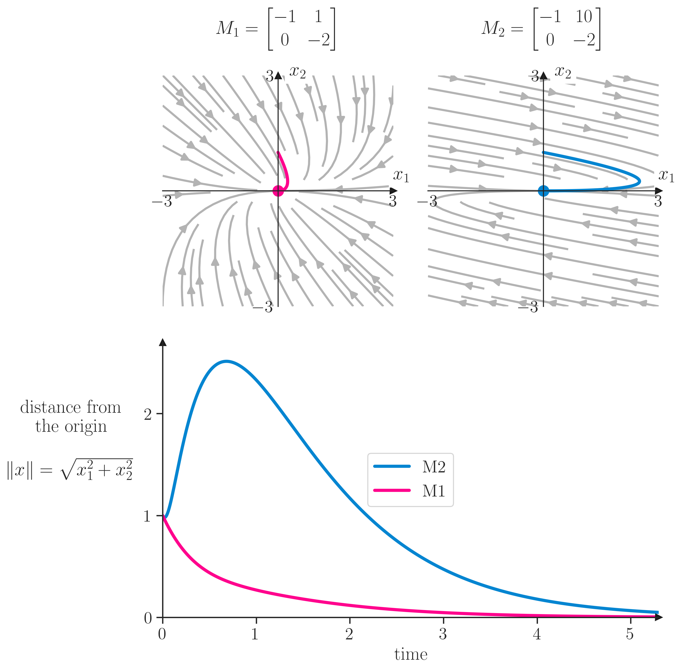
The solution \(\mathbf{x}=(0,0)\) is stable because both eigenvalues of \(M\) are negative. What happens when we change the matrix slightly, but still keeping the eigenvalues exactly the same as before?

# learn how to configure:
# http://matplotlib.sourceforge.net/users/customizing.html
params = {
          'font.family': 'serif',
          'ps.usedistiller': 'xpdf',
          'text.usetex': True,
          # include here any neede package for latex
          'text.latex.preamble': r'\usepackage{amsmath}',
          }
plt.rcParams.update(params)
# matplotlib.rcParams['text.latex.preamble'] = [
#     r'\usepackage{amsmath}',
#     r'\usepackage{mathtools}']

fig = plt.figure(figsize=(10, 10))
gs = gridspec.GridSpec(2, 2, width_ratios=[1,1], height_ratios=[1,1])
gs.update(left=0.20, right=0.86,top=0.88, bottom=0.13, hspace=0.05, wspace=0.15)

ax0 = plt.subplot(gs[0, 0])
ax1 = plt.subplot(gs[0, 1])
ax2 = plt.subplot(gs[1, :])

density = 2 * [0.80]
minlength = 0.2
arrow_color = 3 * [0.7]
bright_color1 = "xkcd:hot pink"
bright_color2 = "xkcd:cerulean"

# make sure that each axes is square
ax0.set_aspect('equal', 'box')
ax1.set_aspect('equal', 'box')

ax0.streamplot(X, Y, system_equations_2d(A1, X, Y)[0], system_equations_2d(A1, X, Y)[1],
              density=density, color=arrow_color, arrowsize=1.5,
              linewidth=2,
              minlength=minlength,
              zorder=-10
              )
ax1.streamplot(X, Y, system_equations_2d(A2, X, Y)[0], system_equations_2d(A2, X, Y)[1],
              density=density, color=arrow_color, arrowsize=1.5,
              linewidth=2,
              minlength=minlength,
              zorder=-10
              )
ax0.plot(t1.y[0], t1.y[1], color=bright_color1, lw=3)
ax1.plot(t2.y[0], t2.y[1], color=bright_color2, lw=3)
ax0.plot(t1.y[0][-1], t1.y[1][-1], 'o', color=bright_color1, markersize=10)
ax1.plot(t2.y[0][-1], t2.y[1][-1], 'o', color=bright_color2, markersize=10)

# make spines at the origin, put arrow at the end of the axis
ax_list = [ax0, ax1]
for axx in ax_list:
    axx.spines['left'].set_position('zero')
    axx.spines['bottom'].set_position('zero')
    axx.spines['right'].set_color('none')
    axx.spines['top'].set_color('none')
    axx.spines['left'].set_linewidth(1.0)
    axx.spines['bottom'].set_linewidth(1.0)
    axx.xaxis.set_ticks_position('bottom')
    axx.yaxis.set_ticks_position('left')
    axx.xaxis.set_tick_params(width=0.5)
    axx.yaxis.set_tick_params(width=0.5)
    # put arrow at the end of the axis
    axx.plot(1, 0, ">k", transform=axx.get_yaxis_transform(), clip_on=False)
    axx.plot(0, 1, "^k", transform=axx.get_xaxis_transform(), clip_on=False)
    axx.text(1, 0.55, r"$x_1$", transform=axx.transAxes, clip_on=False, bbox=dict(facecolor='white', edgecolor='white'))
    axx.text(0.55, 1, r"$x_2$", transform=axx.transAxes, clip_on=False, bbox=dict(facecolor='white', edgecolor='white'))
    # set limits
    axx.set(xticks=[-3,3],
                   yticks=[-3,3],
                   xlim=[-3, 3],
                   ylim=[-3, 3],)
    # remove ticks from both axes
    axx.tick_params(axis='both', which='both', length=0)

# put on title the respective parameters as matrix, use latex equation
# add pad to title to avoid overlap with x-axis
ax0.set_title(r'$M_1=\begin{bmatrix} -1 & 1 \\ 0 & -2 \end{bmatrix}$', pad=40)
ax1.set_title(r'$M_2=\begin{bmatrix} -1 & 10 \\ 0 & -2 \end{bmatrix}$', pad=40)

L2_one = np.sqrt(t1.y[0]**2 + t1.y[1]**2)
L2_two = np.sqrt(t2.y[0]**2 + t2.y[1]**2)


# bottom plot
ax2.plot(t2.t, L2_two, color=bright_color2, lw=3, label='M2')
ax2.plot(t1.t, L2_one, color=bright_color1, lw=3, label='M1')
ax2.legend(loc='center')
ax2.set(xlim=[0,5.3],
        ylim=[0,2.7],
        yticks=[0,1,2],
        xlabel='time',)
ax2.set_ylabel('distance from\nthe origin\n\n' + r"$\lVert x\rVert =\sqrt{x_1^2+x_2^2}$", labelpad=70, rotation=0)
# only left and bottom spines
ax2.spines['right'].set_color('none')
ax2.spines['top'].set_color('none')

ax2.plot(1, 0, ">k", transform=ax2.get_yaxis_transform(), clip_on=False)
ax2.plot(0, 1, "^k", transform=ax2.get_xaxis_transform(), clip_on=False)

resilience

Resilience is defined as the minimal return rate to steady state:

\[ R = -\text{Re}(\lambda_1(M)), \]

where \(\lambda_1(M)\) is the eigenvalue with the largest real part.

mathematical interlude: how to solve the system of equations

The solution of the system of equation goes as follows:

\[ \frac{d\mathbf{x}}{dt} = M \mathbf{x} \Rightarrow \mathbf{x}(t) = e^{Mt} \mathbf{x}_0 \]

Now we need to compute the matrix exponential \(e^{Mt}\). If \(M\) is diagonalizable, then \(M = PDP^{-1}\), where \(D\) is a diagonal matrix with the eigenvalues of \(M\) on the diagonal and \(P\) is the matrix whose columns are the eigenvectors of \(M\):

\[\begin{align*} e^{Mt} =& e^{\left(PDP^{-1}\right)t} \\ =& P e^{Dt} P^{-1} \\ =& P \begin{pmatrix} e^{\lambda_1 t} & 0 \\ 0 & e^{\lambda_2 t} \end{pmatrix} P^{-1} \end{align*}\]

Why do the \(P\) matrices get off the exponential? Because

\[\begin{align*} e^{Mt} &= I + PDP^{-1}t + \frac{1}{2!}PD^2P^{-1}t^2 + \ldots \\ &= P \left( I + Dt + \frac{1}{2!}D^2t^2 \right)P^{-1} \\ &= P e^{Dt} P^{-1} \end{align*}\]

and it is easy to show that

\[ e^{Dt} = \begin{pmatrix} e^{\lambda_1 t} & 0 \\ 0 & e^{\lambda_2 t} \end{pmatrix} \]

Let’s compute the eigenvalues \(M\):

\[\begin{align*} \text{det}(M - \lambda I) &= 0 \\ \text{det} \left[\begin{pmatrix} \lambda_1 & c \\ 0 & \lambda_2\end{pmatrix} - \begin{pmatrix} \lambda & 0 \\ 0 & \lambda\end{pmatrix} \right] &= 0 \\ \text{det} \begin{pmatrix} \lambda_1 - \lambda & c \\ 0 & \lambda_2 -\lambda\end{pmatrix} &= 0 \\ (\lambda_1 - \lambda)(\lambda_2 - \lambda) &= 0 \\ \text{therefore } \lambda &= \lambda_1 \text{ or } \lambda = \lambda_2 \end{align*}\]

Now the eigenvector of \(\lambda_1\):

\[\begin{align*} M \mathbf{v} &= \lambda_1 \mathbf{v} \\ \begin{pmatrix} \lambda_1 & c \\ 0 & \lambda_2 \end{pmatrix} \begin{pmatrix} v_1 \\ v_2 \end{pmatrix} &= \lambda_1 \begin{pmatrix} v_1 \\ v_2 \end{pmatrix} \\ \text{yielding } \lambda_1 v_1 + c v_2 &= \lambda_1 v_1 \\ \lambda_2 v_2 &= \lambda_2 v_2 \\ \text{therefore } \mathbf{v} &= \begin{pmatrix} 1 \\ 0 \end{pmatrix} \\ \end{align*}\]

Now the eigenvector of \(\lambda_2\):

\[\begin{align*} M \mathbf{u} &= \lambda_2 \mathbf{u} \\ \begin{pmatrix} \lambda_1 & c \\ 0 & \lambda_2 \end{pmatrix} \begin{pmatrix} u_1 \\ u_2 \end{pmatrix} &= \lambda_2 \begin{pmatrix} u_1 \\ u_2 \end{pmatrix} \\ \text{yielding } \lambda_1 u_1 + c u_2 &= \lambda_2 u_1 \\ \lambda_2 u_2 &= \lambda_2 u_2 \\ \text{therefore } \mathbf{u} &= \begin{pmatrix} c \\ \lambda_2-\lambda_1 \end{pmatrix} \\ \end{align*}\]

Finally, we found that the matrix \(P\) is:

\[ P = \begin{pmatrix} 1 & c \\ 0 & \lambda_2-\lambda_1 \end{pmatrix} \]

We need \(P^{-1}\), but it’s not fun to compute inverse matrices. In the case where \(\lambda_1=-1\) and \(\lambda_2=-2\), we have:

\[ P = \begin{pmatrix} 1 & c \\ 0 & -1 \end{pmatrix} \]

Now we’re lucky, because it’s easy to see that \(P\) is its own inverse (it’s called an involutory matrix):

\[ PP^{-1} = I \implies \begin{pmatrix} 1 & c \\ 0 & -1 \end{pmatrix}\begin{pmatrix} 1 & c \\ 0 & -1 \end{pmatrix} = \begin{pmatrix} 1 & 0 \\ 0 & 1 \end{pmatrix}_\blacksquare \]

Finally, we have:

\[\begin{align*} \mathbf{x}(t) &= \mathbf{x}_0 e^{Mt} = \begin{pmatrix} 1 & c \\ 0 & -1 \end{pmatrix} \begin{pmatrix} e^{-t} & 0 \\ 0 & e^{-2t} \end{pmatrix} \begin{pmatrix} 1 & c \\ 0 & -1 \end{pmatrix} \mathbf{x}_0 \\ &= \begin{pmatrix} e^{-t} & ce^{-2t} \\ 0 & -e^{-2t} \end{pmatrix} \begin{pmatrix} 1 & c \\ 0 & -1 \end{pmatrix} \mathbf{x}_0 \\ &= \begin{pmatrix} e^{-t} & ce^{-t}-ce^{-2t} \\ 0 & e^{-2t} \end{pmatrix} \mathbf{x}_0 \\ &= \begin{pmatrix} e^{-t} & ce^{-t}-ce^{-2t} \\ 0 & e^{-2t} \end{pmatrix} \begin{pmatrix} x_{01} \\ x_{02} \end{pmatrix} \\ x_1(t) &= x_{01}\, e^{-t} + c\, x_{02} (e^{-t} - e^{-2t}) \\ x_2(t) &= x_{02}\, e^{-2t} \end{align*}\]

the big question for today

The question arises whether asymptotic behavior adequately characterizes the response to perturbations. Because of the short duration of many ecological experiments, transients may dominate the observed responses to perturbations. In addition, transient responses may be at least as important as asymptotic responses. Managers charged with ecosystem restoration, for example, are likely to be interested in both the short-term and long-term effects of their manipulations, particularly if the short-term effects can be large.

Source: Neubert & Caswell, 1997, Ecology

Reactivity

Source: Neubert, M. G., & Caswell, H. (1997). Alternatives to resilience for measuring the responses of ecological systems to perturbations. Ecology, 78(3), 653-665.

The reactivity is defined as the (normalized) maximum rate of change of the norm of the state vector \(\mathbf{x}\), for all nonzero initial conditions:

\[ \sigma \equiv \max_{x_0\neq0} \left[ \left( \frac{1}{\lVert\mathbf{x}\rVert} \frac{d\lVert\mathbf{x}\rVert}{dt} \right)\Bigg|_{t=0} \right] \]

Let’s play with this definition and see what we get.

\[\begin{align*} \frac{d\lVert\mathbf{x}\rVert}{dt} &= \frac{d\sqrt{\mathbf{x}^T\mathbf{x}}}{dt} \\ &= \frac{1}{2}\left( \mathbf{x}^T\mathbf{x} \right)^{-1/2} \frac{d}{dt}\left(\mathbf{x}^T\mathbf{x}\right) \\ &= \frac{1}{2\lVert\mathbf{x}\rVert}\left[ \mathbf{x}^T \frac{d\mathbf{x}}{dt} + \left(\frac{d\mathbf{x}}{dt}\right)^T \mathbf{x} \right] \\ &= \frac{\mathbf{x}^T A \mathbf{x} + \mathbf{x}^T A^T \mathbf{x}}{2\lVert\mathbf{x}\rVert} \\ &= \frac{\mathbf{x}^T \left( A + A^T \right) \mathbf{x}}{2\lVert\mathbf{x}\rVert} \end{align*}\]

The matrix

\[ H(A) = \frac{A + A^T}{2} \]

is called the Hermitian (symmetric) part of \(A\).

The reactivity is then \[ \sigma = \max_{\mathbf{x_0}\neq0} \left[ \frac{\mathbf{x}^T H(A) \mathbf{x}}{\lVert\mathbf{x}\rVert^2} \right]_{t=0} \]

\[ \sigma = \lambda_{\text{max}}(H(A)) \]

In simple words, the reactivity is the maximum eigenvalue of the Hermitian (symmetric) part of the matrix \(A\). Differently from the resilience, the reactivity is always real, because the Hermitian part of a matrix always has real eigenvalues.

If \(\sigma > 0\) then at least one perturbation from the steady state \((\mathbf{x_0}\neq0)\) will grow before it returns to the steady state. If \(\sigma < 0\) then all perturbations \((\mathbf{x_0})\) will decay to the steady state without growing initially.

amplification envelope

\[ \rho(t) = \max_{\mathbf{x_0}\neq0} \frac{\lVert\mathbf{x}\rVert(t)}{\lVert\mathbf{x}_0\rVert} \]

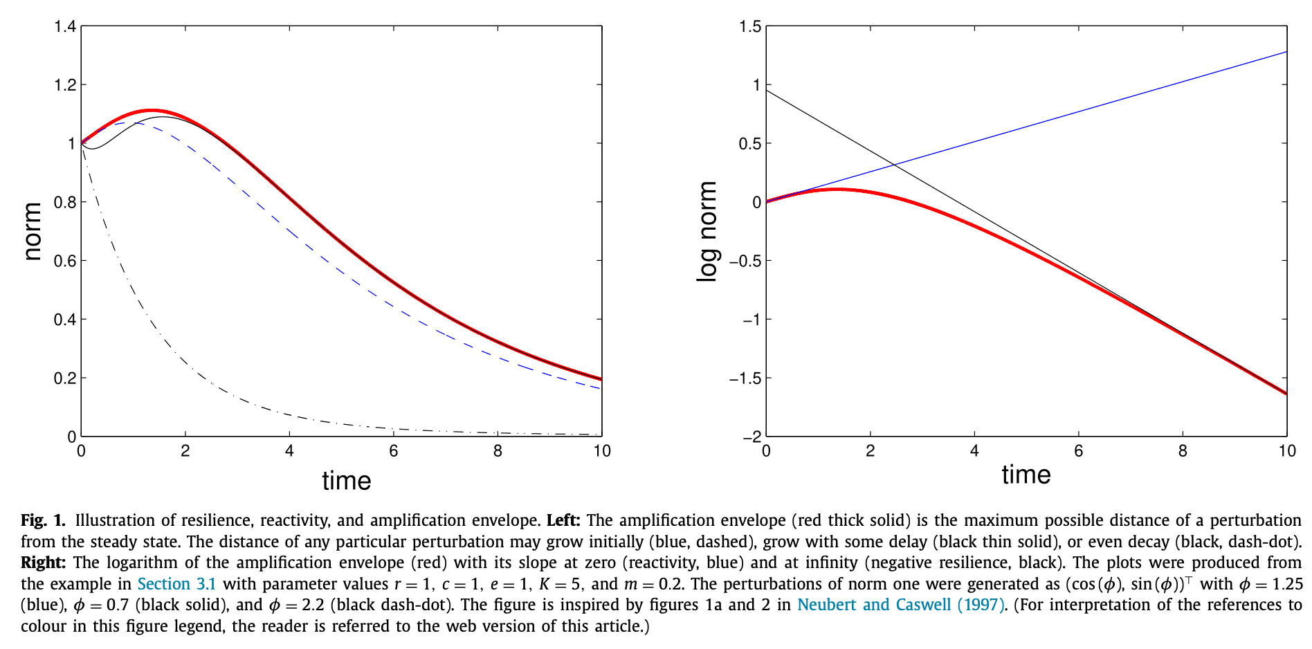
This measures, for any time \(t > 0\), the maximal deviation of any perturbation from the steady state.

Source: Lutscher (2020)

In general, there is not one initial perturbation that follows the amplification envelope all the time. Rather, for different \(t\), different initial perturbations produce the maximum deviation.

From the amplification envelope one can calculate the reactivity and resilience as the slope of \(\ln(\rho(t))\) in the limits as \(t \rightarrow 0\) and \(t \rightarrow \infty\):

\[ \sigma = \frac{d}{dt}\ln\left[\rho(t)\right]\Bigg|_{t=0} \]

\[ R = \frac{d}{dt}\ln\left[\rho(t)\right]\Bigg|_{t=\infty} \]

problem: scaling

The definition of reactivity depends on the norm chosen, whereas resilience and stability do not. In particular, reactivity may depend on scaling.

Solution?

Mari, L., Casagrandi, R., Rinaldo, A., & Gatto, M. (2017). A generalized definition of reactivity for ecological systems and the problem of transient species dynamics. Methods in Ecology and Evolution, 8(11), 1574-1584.

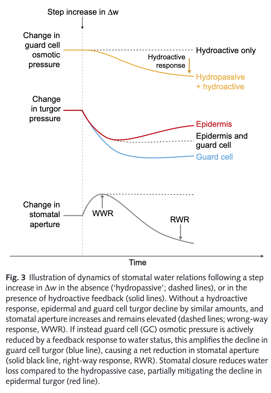
wrong-way response

Source: Buckley, T. N. (2019). How do stomata respond to water status?. New Phytologist, 224(1), 21-36.

Sources

Lutscher, F., & Wang, X. (2020). Reactivity of communities at equilibrium and periodic orbits. Journal of Theoretical Biology, 493, 110240.

Mari, L., Casagrandi, R., Rinaldo, A., & Gatto, M. (2017). A generalized definition of reactivity for ecological systems and the problem of transient species dynamics. Methods in Ecology and Evolution, 8(11), 1574-1584.

McCoy, J. H. (2013). Amplification without instability: applying fluid dynamical insights in chemistry and biology. New Journal of Physics, 15(11), 113036.

Neubert, M. G., & Caswell, H. (1997). Alternatives to resilience for measuring the responses of ecological systems to perturbations. Ecology, 78(3), 653-665.

Verdy, A., & Caswell, H. (2008). Sensitivity analysis of reactive ecological dynamics. Bulletin of Mathematical Biology, 70, 1634-1659.

Vesipa, R., & Ridolfi, L. (2017). Impact of seasonal forcing on reactive ecological systems. Journal of Theoretical Biology, 419, 23-35.